
Mean Reversion Trading System
Mean Reversion Trading System
Many traders who managed to design and implement a mean reversion system ‘correctly’ made a fortune. Fact is that financial markets move in cycles (see 8.6 year cycle – Princeton Economics). In simple words everything that goes up must come down and everything that goes down must come up. Nothing moves in one direction forever. When it comes to the markets we basically have two possible outcomes it’s either trending or the pattern will be defined as a trading range that reverts back to the mean. Our previous research that we did on opening range breakout systems already showed us that opening range breakouts define the trend for the rest of the day in about 30% of the time. Which means that out of 20 trading days we have 6 trending days without price reverting back to a mean. On the other hand we have 70% of the moves that will revert back to the mean several times a day. It’s important to note that the 70 % are referring to intraday price moves. This is something that should ring the alarm bells. 70% of the time the market moves in cycles. Which means that range bound markets are definitely more common.
The first step in building such a system is to define what mean reversion is. Mean reversion systems are looking for markets that are unusually high or low and will eventually return back to the mean. We want a system that looks at a particular market with a significant deviation from their average. The first step to come up with a good trading idea that we can test is to observe the price chart on different time frames. The next step is a quick statistical analysis of our data.
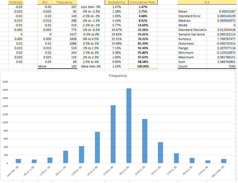
The above data shows us the descriptive statistics of the Russel 2000 Index. In particular we have the measure of central tendency. The mean is calculated by finding the sum of the study data and dividing it by the total number of data. As the data shows most of the time we have a price move between -0.5% and +0.5%. Everything else is defined as an above average standard deviation from the average. These are the moves we will be looking for. We can already come up with a possible setup that must be present before we enter into a position. We are interested in above average price moves which means below -0.5% and above +0.5%. Furthermore we want these price moves to occur early in a trading day since we want to give the market enough time to revert back to the mean. It doesn’t make much sense if this move occurs somewhere at the end of the trading day. It lowers our odds to make a profit due to the fact that we are approaching the market close and volume will dry up (last quantile of a trading day). Another important detail that we need to factor in is the ability of our system to recognize if it’s a trending market or a range bound market. It is important to recognize the trending markets otherwise your system will incur huge losses sooner or later. As a general rule of thumb mean reversion strategies work better on shorter time frames.
Now let’s summarize :
- Move of above average below -0.5% above 0.5%
- Within the first half of a trading day
- Non trending market.
In order to improve the predictability of prevailing market conditions we will use statistical arbitrage of two assets. In our case Russel 2000 and VIX . The basic idea is that some quantities are historically correlated sometimes these correlations are temporarily undone by unusual price moves. The assumption is that these correlations will be restored in the future. Therefore we calculate the relative spread between the Russel 2000 futures contract and the VIX futures contract during the last n number of bars. The look back period will be optimized during our back-tests as we see fit.
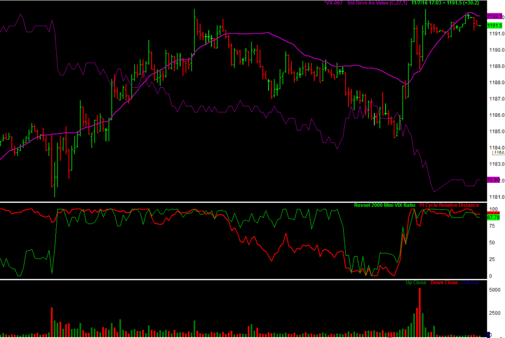
Since these two markets are inversely correlated it makes sense to construct a spread assuming the spread between those two assets converges back to the mean.
Test Results:
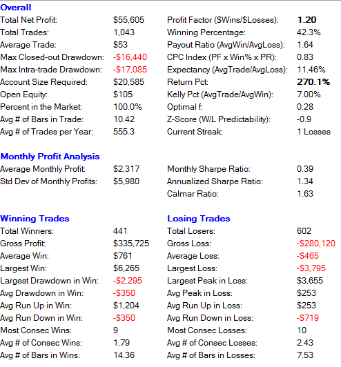
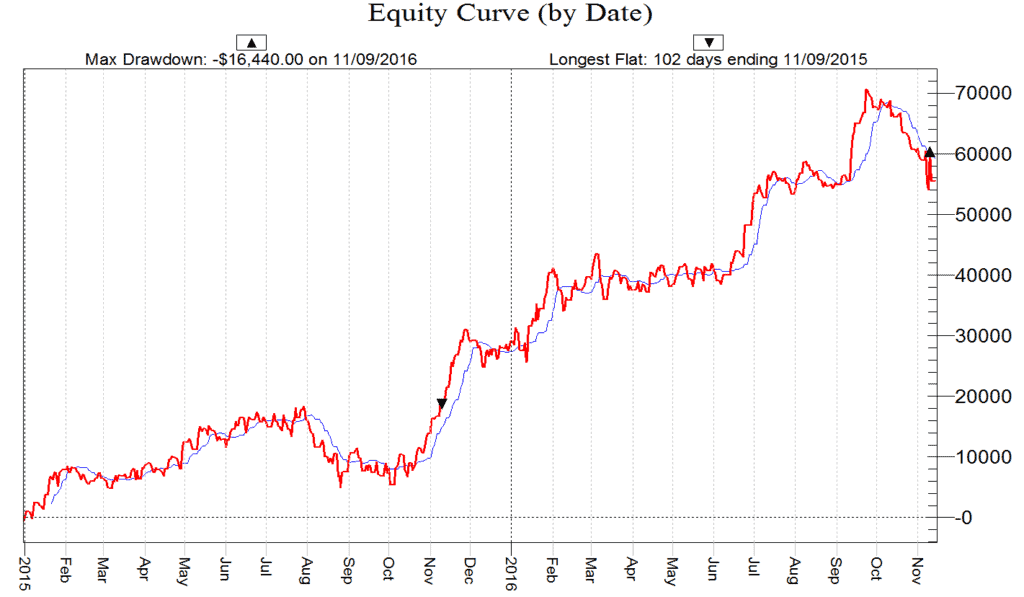
Due to the number of trades we can state that the results are statistically significant. We have no large losses and an acceptable payout ratio of 1.64. The largest consecutive losses occur between Aug 2015 and October 2015. Interestingly enough this was also the period of an elevated VIX level with large intraday spikes. Both assets moved in a more random fashion during this highly volatile period. The divergence and convergence that is typical for range bound markets was invalid for the aforementioned period. Same goes for the month before the elections.
Monte Carlo Analysis
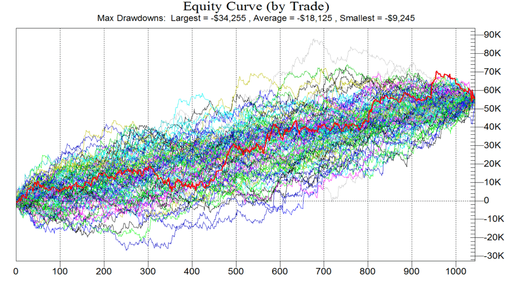
After 10.000 simulations and a random order of trades we can observe that on average (red thick line) the strategy performs positive with no significant losses. However the system needs improvement but it offers a good foundation for further research and the implementation of additional filters.
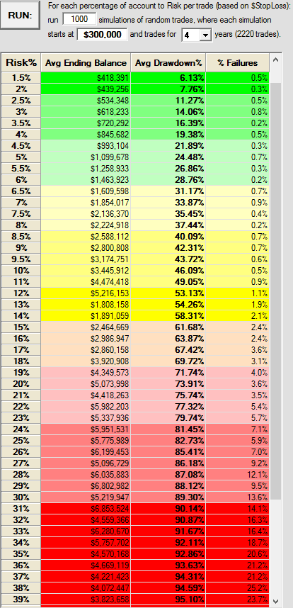
After running the simulations with different risk % we can observe that the average draw-down for 4% risk is only 19,38% which is good considering the fact that the strategy generates a profit of +270% between 2015 and 2016.