


The Complete Guide to Portfolio Optimization in R PART1
Content
PART1:
- Working with data
- Loading times series data sets
- Reading data from CSV files
- Downloading data from the internet
- Modifying time series data
- Sample time series data randomly
- Sorting in ascending order
- Reverse data
- Alignment of timeSeries objects
- Merging time series data
- Binding time series
- Merging columns and rows
- Subsetting data and replacing parts of a data set
- Find first and last records in a time series
- Subset by column names
- Extract specific date
- Aggregating data
- Computing rolling statistics
- Manipulate data with financial functions
- Robust statistical methods
- Implementing the portfolio framework
PART2:
- Representing data with timeSeries objects
- Set portfolio constraints
- Optimizing a portfolio
- Case study portfolio optimization
- Portfolio backtesting
- What to do next
The purpose of portfolio optimization is to minimize risk while maximizing the returns of a portfolio of assets. Knowing how much capital needs to be allocated to a particular asset can make or break an investors portfolio. In this article we will use R and the rmetrics fPortfolio package which relies on four pillars:
- Definition of portfolio input parameters, loading data and setting constraints.
- Optimization of the portfolio.
- Generation of reports and summarizing results.
- Analyzing portfolio performance including backtests.
First we present several aspects of data analysis. It includes a summary on how to modify data sets and how to measure statistical properties. Next we dive into the rmetrics framework used for portfolio selection and optimization. The final part which is presented in part2 of this tutorial is dedicated to mean variance portfolio optimization, mean CVaR portfolios and backtesting. Finally we are putting it all together showing you a portfolio optimization process form A to Z.
This tutorial is aimed towards the practical application of portfolio optimization with R we will not go into theoretical details of every single aspect of portfolio optimization. However, there will be theoretically based explanations on certain parts of the process which we deem important to understand.
Working with data
We start with manipulation of time series data. In case of financial assets the data is usually presented by an S4 timeSeries object in R. We show how to re-sample a time series, reverse it and sort it by ascending and descending time. Financial time series data mainly consists of prices, indexes and derived values, such as volatilities, drawdowns and returns. Rmetrics provides functions to compute such derived series.
To get started we install RStudio which includes a console, syntax-highlighting editor that supports direct code execution, and a variety of tools for plotting, viewing history, debugging and managing your workspace. We recommend installing the following packages: mvoutlier, pastecs, cluster and fPortfolio. To install the packages and all its dependencies we can use the following command in the R environment:
install.packages(c("cluster","mvoutlier","pastecs","fPortfolio"),repos="http://cran.r-project.org")

#To update all packages we run:
update.packages(repos="http://cran.r-project.org")
In our case the data we are working with is represented by a numeric matrix, where each column belongs to the data of an asset. The row belongs to a specific time stamp. The easiest way to represent this data is by a position vector of character strings. When combining the string vector of positions with the numeric matrix of data we can generate timeSeries objects. Rmetrics uses time stamps to create timeDate objects. For the sake of simplicity we use the financial datasets that are provided with the fPortfolio package. The datasets are stored as S4 timeSeries objects and don’t need to be loaded. To use the data sets as CSV files, you can load them as data frames using the data() function in R and convert them into S4 timeSeries objects using the function as.timeSeries().
Data sets used in our tutorial:
- SWX: Daily Swiss equities, bonds and reits time series data.
- LPP2005: Daily pictet swiss pension fund benchmarks
- SPISECTOR: Swiss performance sector indexes
- GCCINDEX: Gulf Cooperation Council equity indexes
- SMALLCAP: Monthly selected US Small Cap equities
- MSFT: Daily data for Microsoft
Loading times series data sets
Below example shows the returns from the daily SWX market indices.
>class(SWX.RET)
[1] "timeSeries"
attr(,"package")
[1] "timeSeries"

>colnames(SWX.RET)
[1] "SBI"  "SPI"  "SII"  "LP25" "LP40" "LP60"

>head(SWX.RET[,1:3])
GMT
                     SBI          SPI           SII
2000-01-04 -0.0020881194 -0.034390059  1.367381e-05
2000-01-05 -0.0001045205 -0.010408271 -4.955306e-03
2000-01-06 -0.0013597617  0.012119128  3.812899e-03
2000-01-07  0.0004185852  0.022461656 -6.162105e-04
2000-01-10  0.0000000000  0.002107677  2.380579e-03
2000-01-11 -0.0010467917 -0.002773654 -2.938453e-04
The third line restricts the output to the first 6 lines of the Swiss Bond Index, Swiss Performance Index and the Swiss Immofunds Index.
Reading data from CSV text files
First we create a small data set using the first 6 lines of the Indexes SBI, SPI and SII. We can use the write.csv() function to write the data to a CSV file. In the current working directory we create the file ‘myData.csv’.
> # create small data set
> data <- head(SWX.RET[, 1:3])
> # write data to a CSV file in the current directory
> write.csv(data, file = "myData.csv")
The data can now be read from our CSV file using the function read-Series().
> # write CSV file in current directory, specifying the separators
> data2 <- readSeries(file = "myData.csv", header = TRUE, sep = ",")
The arguments of the readSeries() function are:
> args(readSeries)
function (file, header = TRUE, sep = ";", zone = "", FinCenter = "",
format, ...)
NULL
Downloading data from the internet
You can use the fImport package which provides functions to download time series data from the internet and make the records available as an S4timeSeries object. For more up to date packages we recomment using quantmod or BatchGetSymbols which will download price data from yahoo finance and organize it so that you don’t need to worry about cleaning the data yourself.
Modifying time series data
We use the daily data sets SWX which contains six financial time series and SWX.RET which contains the daily log returns derived from the SWX data set.
>head(SWX)
GMT
             SBI     SPI     SII  LP25  LP40  LP60
2000-01-03 95.88 5022.86 146.264 99.81 99.71 99.55
2000-01-04 95.68 4853.06 146.266 98.62 97.93 96.98
2000-01-05 95.67 4802.81 145.543 98.26 97.36 96.11
2000-01-06 95.54 4861.37 146.099 98.13 97.20 95.88
2000-01-07 95.58 4971.80 146.009 98.89 98.34 97.53
2000-01-10 95.58 4982.29 146.357 99.19 98.79 98.21

> end(SWX)
GMT
[1] [2007-05-08]

> class(SWX)
[1] "timeSeries"
attr(,"package")
[1] "timeSeries"
The data we load returns an object of class timeSeries. In case we want to rearrange the data we can use rmetrics generic functions :
- sort: sorts a timeSeries in ascending/descending order.
- rev: provided time reversed version of a timeSeries object.
- sample: generates a sample.
Arguments:
- x: an object class timeSeries.
Sample time series data randomly
The sample() function takes a random sample with or without replacement. Below command randomly takes ten rows without replacement from the SWX time series:
> SAMPLE <- sample(SWX[1:10, ])
> SAMPLE
GMT
             SBI     SPI     SII  LP25  LP40  LP60
2000-01-12 95.47 4977.76 146.275 98.91 98.42 97.71
2000-01-13 95.51 4985.22 147.094 99.20 98.81 98.24
2000-01-14 95.65 5042.25 146.940 99.79 99.68 99.52
2000-01-11 95.48 4968.49 146.314 98.95 98.48 97.80
2000-01-06 95.54 4861.37 146.099 98.13 97.20 95.88
2000-01-03 95.88 5022.86 146.264 99.81 99.71 99.55
2000-01-10 95.58 4982.29 146.357 99.19 98.79 98.21
2000-01-07 95.58 4971.80 146.009 98.89 98.34 97.53
2000-01-05 95.67 4802.81 145.543 98.26 97.36 96.11
2000-01-04 95.68 4853.06 146.266 98.62 97.93 96.98
As we can see the data is now not ordered by time.
Sorting in ascending order
> sort(SAMPLE)
GMT
SBI SPI SII LP25 LP40 LP60
2000-01-03 95.88 5022.9 146.26 99.81 99.71 99.55
2000-01-04 95.68 4853.1 146.27 98.62 97.93 96.98
2000-01-05 95.67 4802.8 145.54 98.26 97.36 96.11
2000-01-06 95.54 4861.4 146.10 98.13 97.20 95.88
2000-01-07 95.58 4971.8 146.01 98.89 98.34 97.53
2000-01-10 95.58 4982.3 146.36 99.19 98.79 98.21
2000-01-11 95.48 4968.5 146.31 98.95 98.48 97.80
2000-01-12 95.47 4977.8 146.28 98.91 98.42 97.71
2000-01-13 95.51 4985.2 147.09 99.20 98.81 98.24
2000-01-14 95.65 5042.2 146.94 99.79 99.68 99.52
Reverse data
We can use the function sort(x, decreasing=FALSE), setting the argument decreasing to either FALSE or TRUE:
> rev(sort(SAMPLE))
and
> sort(SAMPLE, decreasing = TRUE)
GMT
             SBI     SPI     SII  LP25  LP40  LP60
2000-01-14 95.65 5042.25 146.940 99.79 99.68 99.52
2000-01-13 95.51 4985.22 147.094 99.20 98.81 98.24
2000-01-12 95.47 4977.76 146.275 98.91 98.42 97.71
2000-01-11 95.48 4968.49 146.314 98.95 98.48 97.80
2000-01-10 95.58 4982.29 146.357 99.19 98.79 98.21
2000-01-07 95.58 4971.80 146.009 98.89 98.34 97.53
2000-01-06 95.54 4861.37 146.099 98.13 97.20 95.88
2000-01-05 95.67 4802.81 145.543 98.26 97.36 96.11
2000-01-04 95.68 4853.06 146.266 98.62 97.93 96.98
2000-01-03 95.88 5022.86 146.264 99.81 99.71 99.55
Alignment of timeSeries objects
Due to public holidays we must expect to have missing data records. If we for example still want to align our times series to a weekly calendar series we need to fill the missing records. The simplest way is to use the price of the previous trading day for the subsequent day. With the function align() the time series data is aligned on calendar dates by default, i.e. on every day of the week. Aligning the SWX time series to daily dates, including holidays and replace the missing values with the price data from the previous trading days can be achieved with the following code:
> nrow(SWX)
[1] 1917
> ALIGNED <- align(x = SWX, by = "1d", method = "before", include.weekends = FALSE)
> nrow(ALIGNED)
[1] 1917
The number of rows shows us that the data does not have missing records. The align function can be used to align daily data sets to weekly data or any arbitrary day of the week using the offset argument.
Merging time series data
To bind different time series together we can use the following functions:
- c: concatenates a timeSeries object.
- cbind: combines a timeSeries by columns.
- rbind: combines a timeSeries by rows.
- merge: merges two timeSeries by common columns and/or rows.
Arguments:
- x,y: objects of class timeSeries.
Here is an example:
> set.seed(1953)
> charvec <- format(timeCalendar(2008, sample(12, 6)))
> data <- matrix(round(rnorm(6), 3))
> t1 <- sort(timeSeries(data, charvec, units = "A"))
> t1
GMT
                A
2008-03-01 -0.733
2008-04-01  1.815
2008-06-01  1.573
2008-09-01 -0.256
2008-10-01 -0.812
2008-12-01  0.289

> charvec <- format(timeCalendar(2008, sample(12, 9)))
> data <- matrix(round(rnorm(9), 3))
> t2 <- sort(timeSeries(data, charvec, units = "B"))
> t2
GMT
                B
2008-01-01  0.983
2008-02-01 -2.300
2008-03-01 -0.840
2008-04-01 -0.890
2008-05-01 -1.472
2008-06-01 -1.307
2008-08-01 -0.068
2008-09-01  0.289
2008-10-01  1.177
> charvec <- format(timeCalendar(2008, sample(12, 5)))
> data <- matrix(round(rnorm(10), 3), ncol = 2)
> t3 <- sort(timeSeries(data, charvec, units = c("A", "C")))
> t3
GMT
                A      C
2008-01-01 -0.649 -0.199
2008-06-01 -0.109 -1.523
2008-07-01  0.318  0.246
2008-08-01  0.796 -2.067
2008-11-01  0.231 -1.001
The t1 and t2 time series are univariate series with 6 ad 9 random records and columns names A and B. The t3 time series is a bivariate series with 5 records per column and column names A and C. The first column A of the t3 time series describes the same time series A as the first series t1.
Binding time series
Functions cbind() and rbind() allow us to bing the time series objects by either column or row. For example, to bind t1 and t2 by columns we can use the following command:
> cbind(t1,t2)
GMT
                A      B
2008-01-01     NA  0.983
2008-02-01     NA -2.300
2008-03-01 -0.733 -0.840
2008-04-01  1.815 -0.890
2008-05-01     NA -1.472
2008-06-01  1.573 -1.307
2008-08-01     NA -0.068
2008-09-01 -0.256  0.289
2008-10-01 -0.812  1.177
2008-12-01  0.289     NA
When using the function rbind() we need to have an equal number of columns in all time series to be bound by rows:
> rbind(t1, t2)
GMT
              A_B
2008-03-01 -0.733
2008-04-01  1.815
2008-06-01  1.573
2008-09-01 -0.256
2008-10-01 -0.812
2008-12-01  0.289
2008-01-01  0.983
2008-02-01 -2.300
2008-03-01 -0.840
2008-04-01 -0.890
2008-05-01 -1.472
2008-06-01 -1.307
2008-08-01 -0.068
2008-09-01  0.289
2008-10-01  1.177
The column name A_B indicates that A and B were bound together.
Merging columns and rows
> tM <- merge(merge(t1, t2), t3)
> tM
GMT
                A      B      C
2008-01-01 -0.649     NA -0.199
2008-01-01     NA  0.983     NA
2008-02-01     NA -2.300     NA
2008-03-01 -0.733 -0.840     NA
2008-04-01  1.815 -0.890     NA
2008-05-01     NA -1.472     NA
2008-06-01 -0.109     NA -1.523
2008-06-01  1.573 -1.307     NA
2008-07-01  0.318     NA  0.246
2008-08-01  0.796     NA -2.067
2008-08-01     NA -0.068     NA
2008-09-01 -0.256  0.289     NA
2008-10-01 -0.812  1.177     NA
2008-11-01  0.231     NA -1.001
2008-12-01  0.289     NA     NA
This gives us a 3 column time series with the time series t1 merged with the first column of t3, both named A, into the same first column of the new time series.
Subsetting data and replacing parts of a data set
The functions for subsetting data sets are as follows:
- [: extracts or replaces subsets by indexes, column
names, date/time stamps, logical predicates, etc - subset: returns subsets that meet specified conditions
- window: extracts a piece between two ‘timeDate’ objects
- start: extracts the first record
- end: extracts the last record
Arguments: - x: an object of class ‘timeSeries’
Subsetting by counts allows us to extract records from rows. For example we can subset a univariate/multivariate timeSeries by row, in our case the second to the fifth row.
> SWX[2:5, ]
GMT
             SBI     SPI     SII  LP25  LP40  LP60
2000-01-04 95.68 4853.06 146.266 98.62 97.93 96.98
2000-01-05 95.67 4802.81 145.543 98.26 97.36 96.11
2000-01-06 95.54 4861.37 146.099 98.13 97.20 95.88
2000-01-07 95.58 4971.80 146.009 98.89 98.34 97.53

> SWX[2:5, 2]
GMT
               SPI
2000-01-04 4853.06
2000-01-05 4802.81
2000-01-06 4861.37
2000-01-07 4971.80

#Since the data is a two dimensional rectangular object
#we need to write SWX[2:5, ] instead of SWX[2:5].
Find first and last records in a time series
To extract the last record of a timeSeries we can use the functions start() and end().
> SWX[start(SWX), ]
GMT
             SBI     SPI     SII  LP25  LP40  LP60
2000-01-03 95.88 5022.86 146.264 99.81 99.71 99.55

> SWX[start(sample(SWX)), ]
GMT
SBI SPI SII LP25 LP40 LP60
2000-01-03 95.88 5022.9 146.26 99.81 99.71 99.55
Subset by column names
With the function tail() we can extract columns by column names.
> tail(SWX[, "SPI"])
GMT
               SPI
2007-05-01 7620.11
2007-05-02 7634.10
2007-05-03 7594.94
2007-05-04 7644.82
2007-05-07 7647.57
2007-05-08 7587.88
Extract specific date
> # Extract a specific date:
> SWX["2007-04-24", ]
GMT
SBI SPI SII LP25 LP40 LP60
2007-04-24 97.05 7546.5 214.91 129.65 128.1 124.34

# Subset all records from Q1 and Q2:
> round(window(SWX, start = "2006-01-15", end = "2006-01-21"), 1)
GMT
SBI SPI SII LP25 LP40 LP60
2006-01-16 101.3 5939.4 196.7 123.1 118.2 110.5
2006-01-17 101.4 5903.5 196.7 123.0 117.9 110.2
2006-01-18 101.5 5861.7 197.2 122.8 117.5 109.5
2006-01-19 101.3 5890.5 198.9 122.9 117.8 110.0
2006-01-20 101.2 5839.4 197.6 122.5 117.3 109.4
Aggregating data
To change the data granularity and go from for example daily data to weekly data we can use the function aggregate() that comes with the R package stats. Using the aggregate() function splits the data sets into two subsets and computes summary statistics for each subset. To illustrate this with an example, let us define a monthly timeSeries that we want to aggregate on a quarterly basis:
> charvec <- timeCalendar()
> data <- matrix(round(runif(24, 0, 10)), 12)
> tS <- timeSeries(data, charvec)
> tS

> tS
GMT
           TS.1 TS.2
2021-01-01    9    5
2021-02-01    5    6
2021-03-01    2    1
2021-04-01    0    3
2021-05-01    4    4
2021-06-01    2    6
2021-07-01    9    7
2021-08-01    2    9
2021-09-01    0    6
2021-10-01    3    9
2021-11-01    8    7
2021-12-01    9    5
Next, the charvec vector searches for the last day in a quarter for each date. We make the breakpoints unique to suppress double dates.
>by <- unique(timeLastDayInQuarter(charvec))
>by
GMT
[1] [2021-03-31] [2021-06-30] [2021-09-30] [2021-12-31]
In a final step the quarterly data series is created with the aggregated monthly data.
>aggregate(tS, by, FUN = sum, units = c("TSQ.1", "TSQ.2"))
GMT
           TSQ.1 TSQ.2
2021-03-31    16    12
2021-06-30     6    13
2021-09-30    11    22
2021-12-31    20    21
To manage special dates we can use the functions included in rmetrics:
- timeLastDayInMonth last day in a given month/year
- timeFirstDayInMonth first day in a given month/ year
- timeLastDayInQuarter last day in a given quarter/year
- timeFirstDayInQuarter first day in a given quarter/year
- timeNdayOnOrAfter date month that is a n-day ON OR AFTER
- timeNdayOnOrBefore date in month that is a n-day ON OR BEFORE
- timeNthNdayInMonth n-th occurrence of a n-day in year/month
- timeLastNdayInMonth last n-day in year/month
We use daily pictet swiss pension fund benchmarks data to illustrate this with another example. The daily returns of the SPI Index are aggregated on monthly periods :
>tS <- 100 * LPP2005.RET[, "SPI"]
>by <- timeLastDayInMonth(time(tS))
>aggregate(tS, by, sum)
GMT
                  SPI
2005-11-30  4.8140571
2005-12-31  2.4812430
2006-01-31  3.1968164
2006-02-28  1.3953612
2006-03-31  2.4826232
2006-04-30  1.4199238
2006-05-31 -5.3718122
2006-06-30  0.5230560
2006-07-31  3.6194503
2006-08-31  2.9160243
2006-09-30  3.2448962
2006-10-31  2.0024849
2006-11-30 -0.5484881
2006-12-31  3.9059090
2007-01-31  4.4125519
2007-02-28 -3.7614955
2007-03-31  2.9538870
2007-04-30  2.0476520
Computing rolling statistics
To cumpute rolling statistics we write a function named rollapply() using the function applySeries().
> rollapply <- function(x, by, FUN, ...)
{
ans <- applySeries(x, from = by$from, to = by$to, by = NULL,
FUN = FUN, format = x@format,
zone = finCenter(x), FinCenter = finCenter(x),
title = x@title, documentation = x@documentation, ...)
attr(ans, "by") <- data.frame(from = format(by$from), to = format(by$to) )
ans
}
We also use the periods function from the timeDate package. The example below demonstrates how to compute returns on a multivariate data set with annual windows and shifted to monthly:
Function:
- periods: constructs equidistantly sized and shifted windows.
Arguments:
- period: size (length) of the periods
- by: shift (interval) of the periods, “m” monthly, “w” weekly, “d” daily, “H” by hours, “M” by minutes, “S” by seconds.
> DATA <- 100 * SWX.RET[, c(1:2, 4:5)]
> by <- periods(time(DATA), "12m", "6m")
> SWX.ROLL <- rollapply(DATA, by, FUN = "colSums")
> SWX.ROLL
GMT
                  SBI        SPI      LP25       LP40
2000-12-31 -0.6487414  11.253322  1.964349  0.8090740
2001-06-30  3.3325805  -5.570437  3.001805  0.5080957
2001-12-31  0.4817268 -24.881298 -1.514506 -4.6842202
2002-06-30  1.4199337 -18.837676 -3.716058 -8.6622991
2002-12-31  6.3741609 -30.045031 -2.177945 -8.7769872
2003-06-30  4.4876745 -18.755693  3.404288  0.4541039
2003-12-31 -1.7801103  19.937351  7.509045 10.1334667
2004-06-30 -3.0571811  19.225778  4.334808  6.7164520
2004-12-31  0.9829797   6.663649  4.773140  5.1319006
2005-06-30  4.4544387  13.157849  9.486836 10.3856460
2005-12-31  0.1678267  30.459956  9.913853 13.5568886
2006-06-30 -5.9878975  22.569102  2.152248  5.0178936
2006-12-31 -3.0139954  18.786250  3.993329  6.1542612
>
Values 12m and 1m in function periods() are called time spans. Another example:
>by <- periods(time(SWX), period = "52w", by = "4w")
The above example rolls on a period of 52 weeks shifted by 4 weeks.
Manipulate data with financial functions
To calculate simple and compound returns we can use the returns() function available in rmetrics. The method argument allows us to define how the returns are computed. Our example below first computes the compound returns for the LP25 benchmark from the SWX data and then cumulates the returns.
> LP25 <- SWX[, "LP25"]/as.numeric(SWX[1, "LP25"])
> head(LP25, 5)
GMT
                LP25
2000-01-03 1.0000000
2000-01-04 0.9880773
2000-01-05 0.9844705
2000-01-06 0.9831680
2000-01-07 0.9907825
> head(returns(LP25), 5)
GMT
                   LP25
2000-01-04 -0.011994298
2000-01-05 -0.003657054
2000-01-06 -0.001323897
2000-01-07  0.007714991
2000-01-10  0.003029081
> head(cumulated(returns(LP25)), 5)
GMT
                LP25
2000-01-04 0.9880773
2000-01-05 0.9844705
2000-01-06 0.9831680
2000-01-07 0.9907825
2000-01-10 0.9937882
> head(returns(cumulated(returns(LP25))), 4)
GMT
                   LP25
2000-01-05 -0.003657054
2000-01-06 -0.001323897
2000-01-07  0.007714991
2000-01-10  0.003029081
Calculating drawdowns
Function:
- durations: computes intervals from a financial series
Arguments:
- x: a ‘timeSeries’ of financial returns
Example for 10 randomly selected records:
>SPI <- SWX[, "SPI"]
>SPI10 <- SPI[c(4, 9, 51, 89, 311, 513, 756, 919, 1235, 1648),
+ ]
>SPI10
GMT
               SPI
2000-01-06 4861.37
2000-01-13 4985.22
2000-03-13 4693.71
2000-05-04 5133.56
2001-03-12 5116.27
2001-12-19 4231.51
2002-11-25 3579.13
2003-07-10 3466.80
2004-09-24 4067.70
2006-04-26 6264.42
Next we compute intervals in units of days:
>durations(SPI10)/(24 * 3600)
GMT
           Duration
2000-01-06       NA
2000-01-13        7
2000-03-13       60
2000-05-04       52
2001-03-12      312
2001-12-19      282
2002-11-25      341
2003-07-10      227
2004-09-24      442
2006-04-26      579
The above code divides the returned value by length of one day. The intervals are especially useful when we want to consider irregular time series and when we want to change data granularity.
We can use the timeSeries objects and add new generic functions. For example, we can add a function to smooth price and index series. We can also add a function to find turnpoints in a time series.
Function
- lowess: a locally-weighted polynomial regression smoother
- turnpoints: finds turnpoints in a financial series
Arguments
- x: a ‘timeSeries’ of financial returns
- f: the smoother span for lowess
- iter: the number of robustifying iterations for lowess
To write a smoother for our data set we can use the lowess() function from the R stats package. With the setMethod() function we can create a formal method for lowess().
>setMethod("lowess", "timeSeries", function(x, y = NULL, f = 2/3,
iter = 3) {
stopifnot(isUnivariate(x))
ans <- stats::lowess(x = as.vector(x), y, f, iter)
series(x) <- matrix(ans$y, ncol = 1)
x
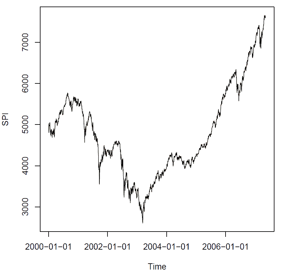
The first thing we need to do is to extract the SPI data from the SWX data set and then smooth the index. With the argument f we determine the smoother span.
> SPI <- SWX[, "SPI"]
> SPI.LW <- lowess(SPI, f = 0.08)
> plot(SPI)
> lines(SPI.LW, col = "brown", lwd = 2)
Output plot:
If we want to find turning points for a financial time series we can use the turnpoints() function available in the pastecs R package. The function enables us to find extrema, i.e. either peaks or troughs:
>library(pastecs)
>setMethod("turnpoints", "timeSeries",
function(x)
{
stopifnot(isUnivariate(x))
tp <- suppressWarnings(pastecs::turnpoints(as.ts(x)))
recordIDs <- data.frame(tp$peaks, tp$pits)
rownames(recordIDs) <- rownames(x)
colnames(recordIDs) <- c("peaks", "pits")
timeSeries(data = x, charvec = time(x),
units = colnames(x), zone = finCenter(x),
FinCenter = finCenter(x),
recordIDs = recordIDs, title = x@title,
documentation = x@documentation)
}
)
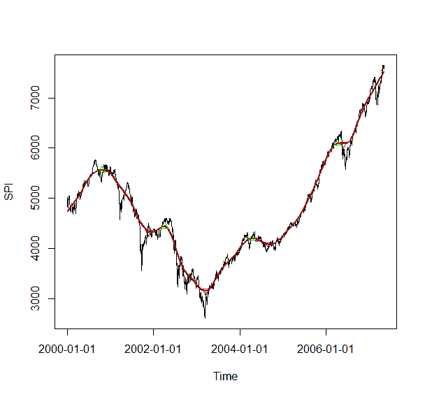
To compute the turning points for the smoothed SPI we do the following:
> SPI.TP <- turnpoints(SPI.LW)
> SPI.PEAKS <- SPI.TP[SPI.TP@recordIDs[, "peaks"] == TRUE, ]
> SPI.PITS <- SPI.TP[SPI.TP@recordIDs[, "pits"] == TRUE, ]
> plot(SPI)
> lines(SPI.LW, col = "brown", lwd = 2)
> points(SPI.PEAKS, col = "green3", pch = 24)
> points(SPI.PITS, col = "red", pch = 25)
Output plot:
Basic statistical analysis with the fPortfolio library
The rmetrics package provides several functions for basic statistical analysis. We can calculate basic statistics, drawdowns, sample mean, covariance estimation and risk estimation, to name a few. For basic statistics we have three functions available: basicStats(), drawdownsStats() and summary().
Create summary statistics and basic statistics report
Summary statistics:
>summary(SWX.RET)
      SBI                  SPI                  SII
 Min.   :-6.868e-03   Min.   :-0.0690391   Min.   :-1.587e-02
 1st Qu.:-7.238e-04   1st Qu.:-0.0047938   1st Qu.:-1.397e-03
 Median : 0.000e+00   Median : 0.0002926   Median : 4.868e-05
 Mean   : 4.661e-06   Mean   : 0.0002153   Mean   : 2.034e-04
 3rd Qu.: 7.847e-04   3rd Qu.: 0.0056807   3rd Qu.: 1.851e-03
 Max.   : 5.757e-03   Max.   : 0.0578604   Max.   : 1.541e-02
      LP25                 LP40                 LP60
 Min.   :-0.0131541   Min.   :-0.0197203   Min.   :-0.0281062
 1st Qu.:-0.0012479   1st Qu.:-0.0019400   1st Qu.:-0.0029165
 Median : 0.0002474   Median : 0.0003514   Median : 0.0004296
 Mean   : 0.0001389   Mean   : 0.0001349   Mean   : 0.0001227
 3rd Qu.: 0.0015866   3rd Qu.: 0.0022826   3rd Qu.: 0.0033255
 Max.   : 0.0132868   Max.   : 0.0211781   Max.   : 0.0320574
Basic report:
> args(basicStats)
function (x, ci = 0.95)
NULL
> basicStats(SWX.RET[, 1:4])
                    SBI         SPI         SII        LP25
nobs        1916.000000 1916.000000 1916.000000 1916.000000
NAs            0.000000    0.000000    0.000000    0.000000
Minimum       -0.006868   -0.069039   -0.015867   -0.013154
Maximum        0.005757    0.057860    0.015411    0.013287
1. Quartile   -0.000724   -0.004794   -0.001397   -0.001248
3. Quartile    0.000785    0.005681    0.001851    0.001587
Mean           0.000005    0.000215    0.000203    0.000139
Median         0.000000    0.000293    0.000049    0.000247
Sum            0.008930    0.412553    0.389689    0.266111
SE Mean        0.000030    0.000248    0.000069    0.000058
LCL Mean      -0.000054   -0.000270    0.000069    0.000025
UCL Mean       0.000063    0.000701    0.000338    0.000253
Variance       0.000002    0.000118    0.000009    0.000006
Stdev          0.001298    0.010843    0.003005    0.002542
Skewness      -0.313206   -0.221507    0.084294   -0.134810
Kurtosis       1.516963    5.213489    2.592051    2.893592
Calculating drawdown statistics:
>args(drawdownsStats)
function (x, ...)
NULL
>LP25 <- SWX.RET[, "LP25"]
>drawdownsStats(LP25)[1:10, ]
         From     Trough         To       Depth Length ToTrough Recovery
1  2001-05-23 2001-09-21 2003-08-22 -0.08470881    588       88      500
2  2006-02-23 2006-06-13 2006-09-04 -0.03874938    138       79       59
3  2001-02-07 2001-03-22 2001-05-17 -0.03113929     72       32       40
4  2004-03-09 2004-06-14 2004-11-12 -0.03097196    179       70      109
5  2000-09-06 2000-10-12 2001-02-06 -0.02103069    110       27       83
6  2005-10-04 2005-10-28 2005-11-24 -0.01821392     38       19       19
7  2003-09-19 2003-09-30 2003-11-03 -0.01743572     32        8       24
8  2000-03-23 2000-05-22 2000-07-11 -0.01732134     79       43       36
9  2000-01-04 2000-01-06 2000-01-17 -0.01691072     10        3        7
10 2000-01-18 2000-02-22 2000-03-17 -0.01668657     44       26       18
Calculate skewness of a time series:
>args(skewness)
function (x, ...)
NULL
>SPI <- SWX[, "SPI"]
>skewness(SPI)
[1] 0.5194545
attr(,"method")
[1] "moment"
If our series has an equal number of large and small amplitude values the skewness is zero. A time series with many small values and few large values is positively skewed and vice versa.
Measuring portfolio risk
Modern portfolio theory dictates that our portfolio includes assets that have a negative covariance. This assumes that the same statistical relationship between the asset prices will continue into the future. To compute the risk measures we can use the three functions covRisk, varRisk and cvarRisk available in the rmetrics package.
> SWX3 <- 100 * SWX.RET[, 1:3]
> covRisk(SWX3, weights = c(1, 1, 1)/3)
      Cov
0.3675482
Value-at- Risk (VaR) is a general measure of risk developed across assets and to aggregate risk on a portfolio basis. VaR is defined as the predicted worst-case loss with a specific confidence level (for example, 95%) over a period of time (for example, one day). For example, J.P. Morgan takes a snapshot of its global trading positions on a daily basis to estimate its DEaR (Daily-Earnings-at-Risk), which is a VaR measure defined as the 95% confidence worst-case loss over the next 24h due to adverse price moves.
>varRisk(SWX3, weights = c(1, 1, 1)/3, alpha = 0.05)
    VaR.5%
-0.5635118
Conditional value at risk is derived from the value at risk for a portfolio. Using CVaR as opposed to just VaR tends to lead to a more conservative approach in terms of risk exposure.
>cvarRisk(SWX3, weights = c(1, 1, 1)/3, alpha = 0.05)
   CVaR.5%
-0.8783248
Robust statistical method
This statistical method produces estimators that are not unduly affected by small departures from model assumptions. The rmetrics package has implemented robust estimators for the mean and covariance of financial assets. The use of statistically robust estimates instead of the widely used classical sample mean and covariance is highly beneficial for the stability properties of the mean-variance optimal portfolios. Many research papers suggest that robust covariance instead of simple covariance achieves a much better diversification of the mean variance portfolio weights.
Robust covariance estimators
The function assetssMeanCov() provides a collection of robust estimators.
Function:
- assetsMeanCov returns robustified covariance estimates
- getCenterRob extracts robust centre estimate
- getCovRob extracts robust covariance estimate
- covEllipsesPlot creates covariance ellipses plot
- assetsOutliers detects multivariate outliers in assets
Arguments:
- x: univariate ‘timeSeries’ object
- method: method of robustification:
- “cov”: uses the sample covariance estimator from [base]
- “mve”: uses the “mve” estimator from [MASS]
- “mcd”: uses the “mcd” estimator from [MASS]
- “MCD”: uses the “MCD” estimator from [robustbase]
- “OGK”: uses the “OGK” estimator from [robustbase]
- “nnve”: uses the “nnve” estimator from [covRobust]
- “shrink”: uses “shrinkage” estimator from [corpcor]
- “bagged”: uses “bagging” estimator from [corpcor]
The following argument lists the methods available:
>args(assetsMeanCov)
function (x, method = c("cov", "mve", "mcd",
    "MCD", "OGK", "nnve", "shrink", "bagged"),
    check = TRUE, force = TRUE, baggedR = 100, sigmamu = scaleTau2,
    alpha = 1/2, ...)
NULL
The “method” argument selects the estimator. The assetsMeanCov() functions returns a named list consisting of four entries center (estimated mean), cov (estimated covariance matrix), mu and Sigma which are synonmys for center and cov. Furthermore, the returned value of the function has a control attrobute attr(), a character vector holding the name of the method of the estimator, and size (number of assets) and two flags. In case of a positive covariance matrix the posdef flag is set to TRUE and vice versa. The functions getCovRob() and getCenterRob() are used to extract the robust mean, center and the robust covariance.
> assetsMeanCov(100 * SWX.RET[, c(1:2, 4:5)], method = "cov")
$center
         SBI          SPI         LP25         LP40
0.0004660521 0.0215319804 0.0138888582 0.0134904088

$cov
              SBI        SPI         LP25         LP40
SBI   0.016851499 -0.0414682 -0.001075973 -0.009441923
SPI  -0.041468199  1.1756813  0.220376219  0.361670440
LP25 -0.001075973  0.2203762  0.064638685  0.099277955
LP40 -0.009441923  0.3616704  0.099277955  0.157780472

$mu
         SBI          SPI         LP25         LP40
0.0004660521 0.0215319804 0.0138888582 0.0134904088

$Sigma
              SBI        SPI         LP25         LP40
SBI   0.016851499 -0.0414682 -0.001075973 -0.009441923
SPI  -0.041468199  1.1756813  0.220376219  0.361670440
LP25 -0.001075973  0.2203762  0.064638685  0.099277955
LP40 -0.009441923  0.3616704  0.099277955  0.157780472

attr(,"control")
 method    size  posdef  forced  forced
  "cov"     "4"  "TRUE" "FALSE"  "TRUE"
>
Comparing robust covariances
With the function covEllipsesPlot() we can visualize differences between two covariance matrices.
Displaying ellipses plots:
>args(covEllipsesPlot)
function (x = list(), ...)
NULL
With the argument method=”mve” we call the minimum volume ellipsoid estimator.
>args(MASS::cov.rob)
function (x, cor = FALSE, quantile.used = floor((n + p + 1)/2),
    method = c("mve", "mcd", "classical"),
    nsamp = "best", seed)
NULL
For our example we invesigate the following indices: SPI, MPI, SBI and LMI. The data is stored in columns 1,2,4,5 of the LPP2005.RET data set.
>set.seed(1954)
>lppData <- 100 * LPP2005.RET[, c(1:2, 4:5)]
>ans.mve <- assetsMeanCov(lppData, method = "mve")
>getCenterRob(ans.mve)
         SBI          SPI          LMI          MPI
-0.004100133  0.140695883  0.001363446  0.124692803
>getCovRob(ans.mve)
             SBI          SPI          LMI         MPI
SBI  0.013407466 -0.011416126  0.008358932 -0.01750865
SPI -0.011416126  0.338050783 -0.006411158  0.19484515
LMI  0.008358932 -0.006411158  0.012777964 -0.01543213
MPI -0.017508646  0.194845146 -0.015432128  0.29530909
>attr(ans.mve, "control")
 method    size  posdef  forced  forced
  "mve"     "4"  "TRUE" "FALSE"  "TRUE"
>
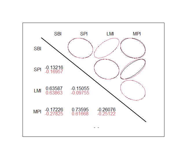
With the function covEllipsesPlot() we can compare the sample covariances woth the “mve” robust covariances.
>covEllipsesPlot(list(cov(lppData), ans.mve$cov))
>title(main = "Sample vs. MVE Covariances")
Output plot:
With the methods “mcd” and “MCD” we can estimate a robust mean and covariance by the minimum covariance determinant estimator. The first method uses the function cov.rob() from the MASS package while the second one uses the function covMcd() from the package robustbase.
>args(MASS::cov.rob)
function (x, cor = FALSE, quantile.used = floor((n + p + 1)/2),
    method = c("mve", "mcd", "classical"),
    nsamp = "best", seed)
NULL
The two estimators can be called and compared as follows:
>ans.mcd <- assetsMeanCov(lppData, "mcd")
>ans.MCD <- assetsMeanCov(lppData, "MCD")
>getCovRob(ans.mcd)
             SBI         SPI          LMI         MPI
SBI  0.013490937 -0.01075959  0.008353551 -0.01332358
SPI -0.010759587  0.33775209 -0.009466100  0.20528659
LMI  0.008353551 -0.00946610  0.012645528 -0.01542817
MPI -0.013323578  0.20528659 -0.015428168  0.32243381
> getCovRob(ans.MCD)
             SBI         SPI          LMI         MPI
SBI  0.015996761 -0.01192936  0.009784193 -0.01605997
SPI -0.011929358  0.40324401 -0.010137846  0.24293820
LMI  0.009784193 -0.01013785  0.014938660 -0.01826193
MPI -0.016059969  0.24293820 -0.018261926  0.37062239
> covEllipsesPlot(list(ans.mcd$cov, ans.MCD$cov))
Implementing the portfolio framework
Another name for portfolio optimization is optimal asset allocation. No matter the name the principles are the same. You want to build a portfolio that yields maximum returns while maintaining the maximum amount of risk you are willing to carry. The end result of your efforts is a portfolio generating the highest possible returns at your established risk tolerance. Whatever your approach is any portfolio optimization strategy will apply the concept of diversification. Diversifying your investments across asset classes is a risk mitigation strategy. Ideally spreading your investments across numerous asset classes allows you to take advantage of different systematic risks. With the rmetrics package we get a set of functions to optimize a portfolio of assets. The goal is to determine the asset weights and minimize the risk for the desired return. Now before we can begin with the optimization process we need to create an environment which specifies a portfolio from the beginning and defines all parameters required for the optimization. With rmetrics we use S4 classes to describe the specification of all parameters of the portfolio, select the assets for which we want to perform the optimization and set the constraints under which the portfolio will be optimized.
Specify a portfolio of assets
The S4 class called fPFOLIOSPEC represents all settings that specify a portfolio of assets.
>showClass("fPFOLIOSPEC")
Class "fPFOLIOSPEC" [package "fPortfolio"]

Slots:

Name:      model portfolio     optim  messages      ampl
Class:      list      list      list      list      list
fPFOLIOSPEC has four slot names @portfolio, @model, @optim and @messages.
- @portfolio: portfolio information and results.
- @model: holds the model information .
- @optim: information about solver used for the optimization.
- @messages: list of optional messages.
With the portfolioSpec() function we define specification settings. The default settings are for a mean variance portfolio. The function formals() prints an easy to read summary of the formal arguments.
>formals(portfolioSpec)
$model
list(type = "MV", optimize = "minRisk", estimator = "covEstimator",
    tailRisk = list(), params = list(alpha = 0.05))

$portfolio
list(weights = NULL, targetReturn = NULL, targetRisk = NULL,
    riskFreeRate = 0, nFrontierPoints = 50, status = NA)

$optim
list(solver = "solveRquadprog", objective = c("portfolioObjective",
    "portfolioReturn", "portfolioRisk"), options = list(meq = 2),
    control = list(), trace = FALSE)

$messages
list(messages = FALSE, note = "")

$ampl
list(ampl = FALSE, project = "ampl", solver = "ipopt",
    protocol = FALSE, trace = FALSE)
The setting are created when we specify the values for portfolio, model, optim and messages. Other arguments of the function portfolioSpec() are listed below.
Arguments:
- model slot
- type = “MV” a string value
- optimize = “minRisk” a string value
- estimator = “covEstimator” a function name
- tailRisk = list() a list
- params =
list(alpha=0.05, a=1, …) a list
portfolio slot: a list
- weights = NULL a numeric vector
- targetReturn = NULL a numeric value
- targetRisk = NULL a numeric value
- riskFreeRate = 0 a numeric value
- nFrontierPoints = 50 an integer value
- status = NA) a integer value
optim slot: a list
- solver = “solveRquadprog” a function names
- objective = NULL function names
- options = list() a list with parameters
- control = list() a list with controls
- trace = FALSE) a logical
messages slot: a list
- list = list() a list
To create a mean variance portfolio with the default settings we call function portfolioSpec() without arguments.
To create a CVaR portfolio we specify at least model type and solver.
>cvarSpec <- portfolioSpec(
model = list(type = "CVaR", optimize = "minRisk",
estimator = "covEstimator", tailRisk = list(),
params = list(alpha = 0.05)),
portfolio = list(weights = NULL,
targetReturn = NULL, targetRisk = NULL,
riskFreeRate = 0, nFrontierPoints = 50,
status = 0),
optim = list(solver = "solveRglpk", objective = NULL,
params = list(), control = list(), trace = FALSE))
To display the structure of a portfolio we can call the function str(). It displays the internal structure of the portfolio specification object.
>str(defaultSpec)
Formal class 'fPFOLIOSPEC' [package "fPortfolio"] with 5 slots
  ..@ model    :List of 5
  .. ..$ type     : chr "MV"
  .. ..$ optimize : chr "minRisk"
  .. ..$ estimator: chr "covEstimator"
  .. ..$ tailRisk : list()
  .. ..$ params   :List of 1
  .. .. ..$ alpha: num 0.05
  ..@ portfolio:List of 6
  .. ..$ weights        : NULL
  .. ..$ targetReturn   : NULL
  .. ..$ targetRisk     : NULL
  .. ..$ riskFreeRate   : num 0
  .. ..$ nFrontierPoints: num 50
  .. ..$ status         : logi NA
  ..@ optim    :List of 5
  .. ..$ solver   : chr "solveRquadprog"
  .. ..$ objective: chr [1:3] "portfolioObjective" "portfolioReturn" "portfolioRisk"
  .. ..$ options  :List of 1
  .. .. ..$ meq: num 2
  .. ..$ control  : list()
  .. ..$ trace    : logi FALSE
  ..@ messages :List of 2
  .. ..$ messages: logi FALSE
  .. ..$ note    : chr ""
  ..@ ampl     :List of 5
  .. ..$ ampl    : logi FALSE
  .. ..$ project : chr "ampl"
  .. ..$ solver  : chr "ipopt"
  .. ..$ protocol: logi FALSE
  .. ..$ trace   : logi FALSE
With the pring() function we print the porfolio specification object.
>print(cvarSpec)

Model List:
 Type:                      CVaR
 Optimize:                  minRisk
 Estimator:                 covEstimator
 Params:                    alpha = 0.05

Portfolio List:
 Target Weights:            NULL
 Target Return:             NULL
 Target Risk:               NULL
 Risk-Free Rate:            0
 Number of Frontier Points: 50
 Status:                    0

Optim List:
 Solver:                    solveRglpk
 Objective:                 list()
 Trace:                     FALSE
With the @model slot we can specify the portfolio settings. It includes the objective function to be optimized, the type of portfolio, estimators for mean and covariance, tail risk and optional model parameters.
Model Slot – Extractor Functions:
- getType Extracts portfolio type from specification
- getOptimize Extracts what to optimize from specification
- getEstimator Extracts type of covariance estimator
- getTailRisk Extracts list of tail dependency risk matrices
- getParams Extracts parameters from specification
With the following functions we can modify the settings from a portfolio specification.
Model Slot – Constructor Functions:
- setType Sets type of portfolio optimization
- setOptimize Sets what to optimize, min risk or max return
- setEstimator Sets names of mean and covariance estimators
- setParams Sets optional model parameters
The list entry $type from the @model slot describes the type of desired portfolio which can take different values.
Model Slot – Argument: type
Values:
- “MV” mean-variance (Markowitz) portfolio
- “CVAR” mean-conditional Value at Risk portfolio
- “QLPM” mean-quadratic-lower-partial-moment portfolio
- “SPS” Stone, Pedersen and Satchell type portfolios
- “MAD” mean-absolute-deviance Portfolio
With setType() we can modify the selection and the getType() function retreives the current settings.
>mySpec <- portfolioSpec()
>getType(mySpec)
[1] "MV"
>setType(mySpec) <- "CVAR"
Solver set to solveRquadprog
>getType(mySpec)
[1] "CVAR"
In the example above we changed the specification from mean variance portfolio to mean conditional value at risk portfolio.
Choosing an objective when optimizing a portfolio
With the list entry $optimize from the @model slot we can choose which objective function to optimize.
Model Slot – Argument: optimize
Values:
- “minRisk” minimizes the risk for a given target return
- “maxReturn” maximizes the return for a given target risk
- “objRisk” gives the name of an alternative objective function
The target return is computed by the sample mean if not otherwise specified. The objRisk function leaves it free to define any portfolio objective function. For example, maximizing the Sharpe ratio. The getOptimize() function is used to retrieve the assignment function setOptimize() to modify the settings.
Estimating mean and covariance of asset returns
The covariance matrix is arguably one of the most important objects when it comes to Modern Portfolio Theory. Typically the covariance matrix is unknown and must be estimated from the data. Besides the default function covEstimator() to compute the sample column means and the sample covariance matrix the rmetrics package offers a number of alternative estimators, like Kendall’s and Spearman’s rank based covariance estimators, shrinkage and bagged estimator, among others. The bagged estimator uses bootstrap aggregating to improve models in terms of stability and accuracy.
Model slot of function portfolioSpec()
Function:
portfolioSpec specifies a portfolio
Model Slot: specifies the type of estimator
List Entry:
estimator
- “covEstimator” Covariance sample estimator
- “kendallEstimator” Kendall’s rank estimator
- “spearmanEstimator” Spearman’s rank estimator
- “mcdEstimator” Minimum covariance determinant estimator
- “mveEstimator” Minimum volume ellipsoid estimator
- “covMcdEstimator” Minimum covariance determinant estimator
- “covOGKEstimator” Orthogonalized Gnanadesikan-Kettenring
- “shrinkEstimator” Shrinkage estimator
- “baggedEstimator” Bagged Estimator
- “nnveEstimator” Nearest neighbour variance estimator
Working with tail risk
Tails risk arises when an investment moves more than three standard deviations from the mean. It includes events that have a small probability of occurring. The concept suggests that the distribution of returns is not normal, but has fatter tails. As explained by Taleb (2019) “Black Swans are not more frequent, they are more consequential. The fattest tail distribution has just one very large extreme deviation, rather than many departures form the norm. …if we take a distribution like the Gaussian and start fattening it, then the number of departures away from one standard deviation drops. The probability of an event staying within one standard deviation of the mean is 68 per cent. As the tails fatten, to mimic what happens in financial markets for example, the probability of an event staying within one standard deviation of the mean rises to between 75 and 95 per cent. So note that as we fatten the tails we get higher peaks, smaller shoulders, and a higher incidence of a very large deviation.”
In rmetrics we can incorporate tail risk calculations by using the list entry tailRisk from the @model slot. It is used to add tail risk budget constraints to the optimization process. For this to work a square matrix of pairwise tail dependence coefficients has to be specified as a list entry. The function getTailRisk() inspects the current setting and setTailRisk() assigns a tail risk matrix.
Set and modify portfolio parameters
To specify the parameters for our portfolio we use the slot @portfolio. It includes the weights, target return, risk, risk free rate, status of the solver and the number of frontier points. With the extractor functions we can retrieve the current settings of the portfolio.
Portfolio Slot – Extractor Functions:
- getWeights: Extracts weights from a portfolio object
- getTargetReturn: Extracts target return from specification
- getTargetRisk: Extracts target risk from specification
- getRiskFreeRate: Extracts risk-free rate from specification
- getNFrontierPoints: Extracts number of frontier points
- getStatus: Extracts the status of optimization
- setWeights Sets weights vector
- setTargetReturn Sets target return value
- setTargetRisk Sets target risk value
- setRiskFreeRate Sets risk-free rate value
- setNFrontierPoints Sets number of frontier points
- setStatus Sets status value
To set the values of weights, target return and risk we use the list entries from the @portfolio slot.
Portfolio slot – Arguments:
- weights a numeric vector of weights
- targetReturn a numeric value of the target return
- targetRisk a numeric value of the target risk
Target return and target risk are determined if the weights for a portfolio are given. If we set the weights to a new value it also changes target return and target risk. Since we don’t know these values in advance, when resetting the weights, target risk and target return are set to NA. The default setting for all three values is NULL. In this case an equal weights portfolio is calculated. If one value is different from NULL, then the following modus operandi will be started:
- a feasible portfolio is considered if weights are specified.
- the efficient portfolio with minimal risk is considered if the target return is fixed.
- if risk is fixed the return is maximized.
The functions setWeights(), setTargetReturn() and setTargetRisk() modify the selection.
Example:
#Load required package: timeSeries
#Load required package: timeDate
#Load required package: fPortfolio
#Load required package: fBasics
#Load required package: fAssets
>library(fPortfolio)
>mySpec <- portfolioSpec()
>getWeights(mySpec)
NULL
>getTargetReturn(mySpec)
NULL
>getTargetRisk(mySpec)
NULL
>setWeights(mySpec) <- c(1, 1, 1, 1)/4
>getWeights(mySpec)
[1] 0.25 0.25 0.25 0.25
>getTargetReturn(mySpec)
[1] NA
>getTargetRisk(mySpec)
[1] NA
>getOptimize(mySpec)
[1] "minRisk"
#Target return and target risk are set to NA, since we don't know the
#return and risk of the equal weights portfolio. If we want to fix target return, for example to 2.5%, we can proceed as follows:
>setTargetReturn(mySpec) <- 0.025
>getWeights(mySpec)
[1] NA
>getTargetReturn(mySpec)
[1] 0.025
>getTargetRisk(mySpec)
[1] NA
>getOptimize(mySpec)
[1] "minRisk"
#Weights and target risk are set to NA, since they are unknown. The #getOptimize() function returns "minRisk", since we specified the #target return. If we set the target risk, for example to 30%, we #obtain the following settings:
>setTargetRisk(mySpec) <- 0.3
>getWeights(mySpec)
[1] NA
>getTargetReturn(mySpec)
[1] NA
>getTargetRisk(mySpec)
[1] 0.3
>getOptimize(mySpec)
[1] "maxReturn"
>
In Part2 of our tutorial we dive into mean variance portfolio optimization, mean CVaR portfolios and backtesting with real world case studies. As mentioned in the beginning we will put it all together showing you a portfolio optimization process form A to Z. If you make your way to the end of this lengthy tutorial (Part1&2) you should be able to:
- understand the concept of portfolio diversification and its benefits for risk-management.
- compute mean-variance portfolios.
- construct ‘optimal’ portfolios.
- backtest and evaluate the performance of ‘optimal’ portfolios.
- understand the limitations of portfolio optimization (Are these portfolios really optimal? When should we rebalance our portfolio? )
For those of you who want to go into even more detail regarding the rmetrics package we recommend reading “Portfolio Optimization with R/Rmetrics”.
——————
References
Bacon, C. R. (2008). Practical Portfolio Performance Measurement and
Attribution (2 ed.). JohnWiley & Sons.
DeMiguel, V.; Garlappi, L.; and Uppal, R. (2009) . “Optimal versus Naive Diversification: How Inefficient Is the 1/N Portfolio Strategy?”. The Review of Financial Studies, pp. 1915—195.
DiethelmWürtz, Tobias Setz,William Chen, Yohan Chalabi, Andrew Ellis (2010). “Portfolio Optimization with R/Rmetrics”.
Guofu Zhou (2008) “On the Fundamental Law of Active Portfolio Management: What Happens If Our Estimates Are Wrong?” The Journal of Portfolio Management, pp. 26-33
Taleb N.N. (2019). The Statistical Consequences of Fat Tails (Technical Incerto Collection)
Würtz, D. & Chalabi, Y. (2009a). The fPortfolio Package. cran.r-project.org.
Wang, N. &Raftery, A. (2002). Nearest neighbor variance estimation (nnve):
Robust covariance estimation via nearest neighbor cleaning. Journal of
the American Statistical Association, 97, 994–1019.