

Pairs Trading – A Real-World Profitable Strategy
Pairs trading is popular due to its simple approach and effectiveness. At the heart of the strategy is how the prices of two assets diverge and converge over time. Pairs trading algorithms profit from betting on the fact that spread deviations return to their mean.
One of the more notable hedge funds that implemented a pairs trading strategy was Long Term Capital Management. The company was founded in 1994 by John Meriwether, the former head of bond trading at Salomon Brothers. Members of LTCM’s board of directors included Myron Scholes and Robert C. Merton, who shared the 1997 Nobel Memorial Prize in Economic Sciences for having developed the Black–Scholes model of financial dynamics.
LTCM was initially successful and a bright star on Wall Street at that time, with annualized returns (after fees) of around 21% in year one, 43% in year two and 41% in its third year. However, in 1998 the fund lost a staggering $4.6 billion in less than four months due to a combination of high leverage and exposure to the 1997 Asian financial crisis and 1998 Russian debt crisis. Why are we telling you this? Well, before diving into the details of the strategy we want you to be aware of the risks involved in such a strategy. Market events as well as poor statistical modeling and parameter estimation may all erode potential profits.
You must therefore take into account three important factors:
- Market events
- Parameter estimation
- Statistical modeling
Depending on the pair you trade you must define market events that can make random departures from equilibrium pricing between two assets not temporary but rather permanent. The LTCM fiasco should give you some guidance on this. Parameters must be adjusted in certain intervals. So, how often should I do this? The answer to that depends on the optimization and walk-forward windows during your initial backtesting of the strategy. If for example the walk-forward window is nine months then the model must be reoptimized after nine months of trading. Considering the risks involved, the statistical arbitrage strategy should have a risk limiting component. Extensive numerical simulations are necessary to derive to the optimal stop loss in case our two assets do not return to equilibrium pricing after a certain time period.
The key challenges are to find a good pair for trading, optimal entry/exit and a stop loss as an additional risk management component.
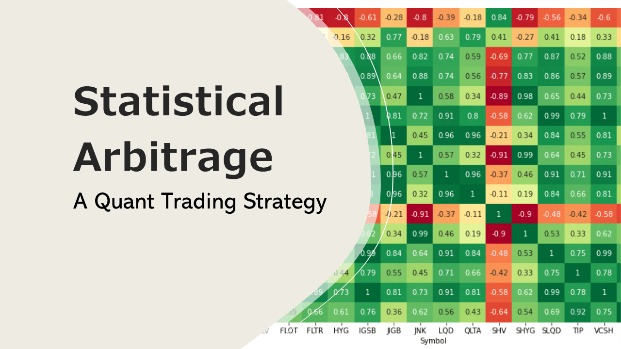
Statistics of Pairs Trading
A pairs trading strategy is based on statistical concepts like mean reversion and stationary stochastic processes. We start our research by looking at correlation and co-integration between two assets. We then try to get a stationary relation that we can transform into an alpha generating trading strategy. Below plot shows a correlation matrix.
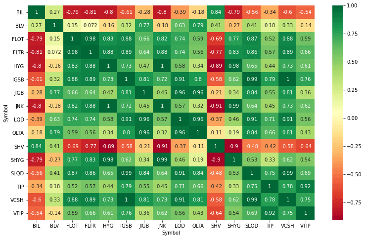
For our strategy we don’t want to look at the correlation alone but at co-integration as well. The co-integration test identifies scenarios where two non-stationary time series are integrated together in a way that they cannot deviate from equilibrium in the long term.
Popular tests for co-integration are Johansen Test and the Augmented Dickey-Fuller (ADF) test. The ADF test enables one to test for cointegration between two-time series. The Johansen Test can test for cointegration between a maximum of 12-time series. With such a test we can create a stationary linear combination of assets using more than two-time series.
Johansen test in python.
Example #1
import numpy as np
import pandas as pd
import statsmodels.api as sm

data = pd.read_csv("http://web.pdx.edu/~crkl/ceR/data/usyc87.txt",index_col='YEAR',sep='\s+',nrows=66)
y = data['Y']
c = data['C']

from statsmodels.tsa.vector_ar.vecm import coint_johansen

"""
    Johansen cointegration test of the cointegration rank of a VECM

    Parameters
    ----------
    endog : array_like (nobs_tot x neqs)
        Data to test
    det_order : int
        * -1 - no deterministic terms - model1
        * 0 - constant term - model3
        * 1 - linear trend
    k_ar_diff : int, nonnegative
        Number of lagged differences in the model.
"""

def joh_output(res):
    output = pd.DataFrame([res.lr2,res.lr1],
                          index=['max_eig_stat',"trace_stat"])
    print(output.T,'\n')
    print("Critical values(90%, 95%, 99%) of max_eig_stat\n",res.cvm,'\n')
    print("Critical values(90%, 95%, 99%) of trace_stat\n",res.cvt,'\n')


# Model 3 (2 lag-difference used = 3 lags VAR or VAR(3) model)
# with constant/trend (deterministc) term
joh_model3 = coint_johansen(data,0,2) # k_ar_diff +1 = K
joh_output(joh_model3)

# Model 2: with linear trend only
joh_model2 = coint_johansen(data,1,2) # k_ar_diff +1 = K
joh_output(joh_model2)

# Model 1: no constant/trend (deterministc) term
joh_model1 = coint_johansen(data,-1,2) # k_ar_diff +1 = K
joh_output(joh_model1)
Example #2
import matplotlib.pyplot as plt
import pandas as pd
from johansen import coint_johansen

df_x = pd.read_csv ("yourfile.csv",index_col=0)
df_y = pd.read_csv ("yourfile.csv",index_col=0)

df = pd.DataFrame({'x':df_x['Close'],'y':df_y['Close']})

coint_johansen(df,0,1)
So far we have discussed the statistical challenges that come with finding the right pair to trade. By using the co-integration test we can say that the spread between two assets is mean reverting. In our next step we define the extreme points which when crossed by this signal, we trigger trading orders for our pairs trading strategy. To identify these points, a statistical construct called z-score is used.
Z-score
The z-score is calculated from raw data points of our distribution so that the new distribution is a normal distribution with mean 0 and standard deviation of 1. With this distribution we can create threshold levels such as 2 sigma, 3 sigma, and so on.
Formula for the z-score:
***
z= (x-mean)/standard deviation
***
Strategy entry points
Spread=s = log(a)-nlog(b)
Calculate z-score of s, using rolling mean and standard deviation for a time period of t intervals (moving average). The calculated value is our z. The threshold parameters are adjusted according to the backtest results.
When Z-score crosses upper threshold:
Short asset A // Long asset B
When Z-score crosses lower threshold:
Long asset A // Short asset B
Strategy exit points
If the spread continues to blow up we use either a stop loss or a sigma value triggering the exit condition. The condition and exact setup is defined during optimization.
Description Test Framework
| Pair | E-mini S&P 500 / T-Bond 30Yr |
| Symbol Traded | E-mini S&P 500 Futures Contract |
| Interval | Daily |
| Start Date | 01/03/2018 |
| End Date | 04/30/2021 |
| Out-of-sample Start | 01/05/2015 |
| Out-of-sample End | 12/29/2017 |
| Contracts | 1 |
| Stop Loss Test Interval | 1000-4000 |
| Stop Loss Test Step Size | 200 |
| Upper Threshold Test Interval | 1-3 |
| Lower Threshold Test Interval | 1-3 |
| Threshold Test Interval Step Size | 0.1 |
After running the optimization we get the following results.
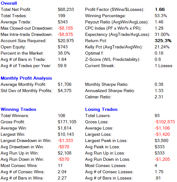
Backtest Results for time period 01/03/2018 – 04/30/2021
Optimized parameters
| Stop Loss | 1400 |
| Upper Threshold | 1.5 |
| Lower Threshold | 1.2 |
| Bars Moving Average (Rolling mean & SD for a time period of t intervals) | 4 |
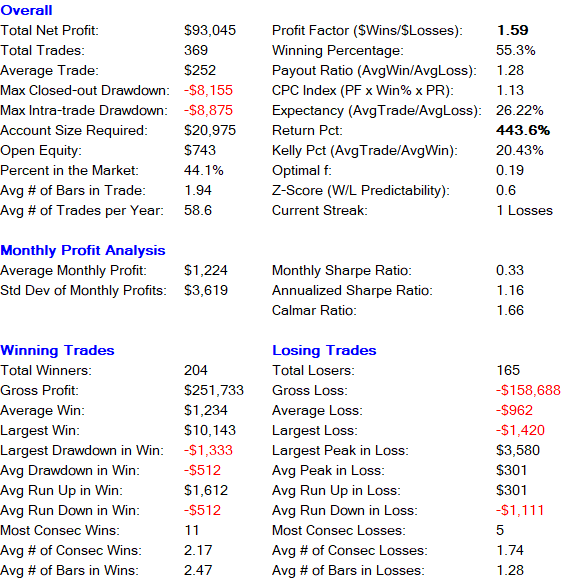
The strategy is profitable in all years. We get the highest return in 2020 with 186.44%. Most of the profit comes from the long side, 267.6%. Short entries give us a return of 72.8%. The recommended account size for the strategy is $20,000 per contract traded.
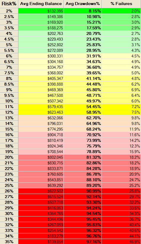
Monte Carlo Simulation
Running 1,000 simulations of random trades where each simulation starts with $100,000 and trades for four years gives us the following risk profile.
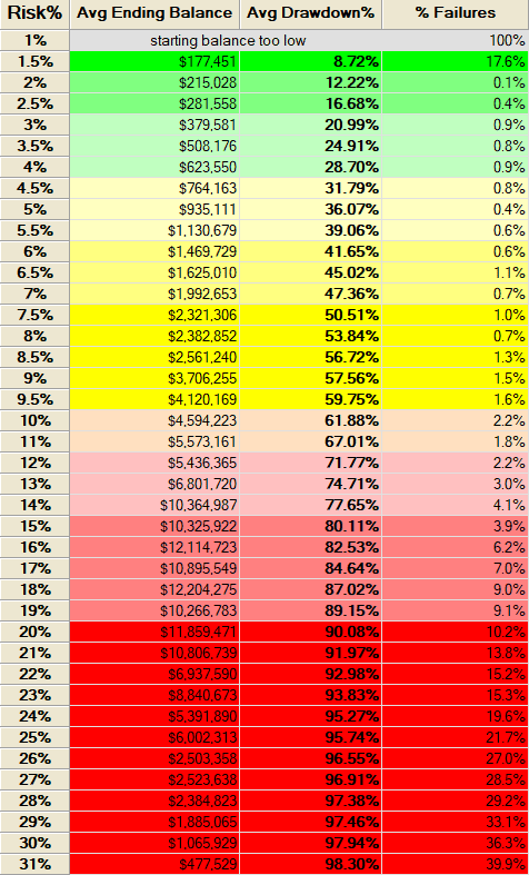
Our sweet spot is around 4%. Assuming we risk 4% per trade, we can trade 3 contracts with a starting capital of $100,000. The average drawdown is 30%. Let’s move on to the walk-forward analysis using the same parameters as before.
Walk-Forward Analysis
There is no better way then WFA to avoid curve fitting. It works by dividing the data into several training and validation sets, and then walks through these sets by optimizing for the best values on the training sets. The best values are applied to the validation set. In our example we use one training set from 2018 to 2021 and one validation set from 2015 to 2017.
The validation set gives us a return of 124.5% with a winning percentage of 57.4%. Here is a detailed breakdown of the strategy performance:
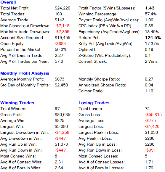
The monte carlo simulation shows an average drawdown of 20% if we risk 4% per trade. The probability of blowing up our account is 2.7%. Again, we have no losing year and the winning percentage as well as the average payout ratio are both consistent across the complete validation set.
Performance Summary In-sample and Out-of-sample
***
Download Trade by Trade Data for further Analysis
***
Conclusion
The strategy shows consistent alpha for in-sample and out-of-sample backtests. The risk profile allows the strategy to perform even better. Nevertheless, we have chosen a more conservative approach with a risk of 4% per trade since the risk of ruin is on average only 1.8% when combining both data sets – training data and validation data.
By understanding the concept of correlation and co-integration we find that trading a suitably formed pair of assets exhibits profits, which are robust to estimates of volatility. The strategy accounts for market events and uncertainty. We have accomplished this in a simple but effective way by adding another stop loss component to our trading strategy. As the results show there is an increase in buyer initiated trades (seller initiated trades) in the underpriced (overpriced) asset when mispricing occurs as arbitragers seek to profit from the mispricing between the E-mini S&P 500 and T-Bond 30Yr futures. Arbitrage opportunities are more likely to be created when the market is more volatile.
Disclaimer
The information on this site is provided for statistical and informational purposes only. Nothing herein should be interpreted or regarded as personalized investment advice or to state or imply that past results are an indication of future performance. Under no circumstances does this information represent an advice or recommendation to buy, sell or hold any security.