
How to develop, test and optimize a trading strategy – complete guide

Content
- Intro
- Elements of a Trading Strategy
- Manage Profit with Exit Orders
- Mind Opening and Closing Slippage
- Limit Move Circuit Breaker and Economic Events
- Expiration and Contract Roll
- Historical Data Backtesting Period
- From Idea and Code to Preliminary Testing
- Optimization Process
Intro
Developing a trading strategy from start to finish is a complex process. The process follows the following steps:
- Formulation of the strategy
- Write Pseudo Code
- Transform into working code
- Start first backtests
- Optimize
- Evaluate test results
- Go live
- Monitor performance
- Evaluate and adjust
- Optimization process
We will discuss each of this points separately. Here is a visualization of the design process:
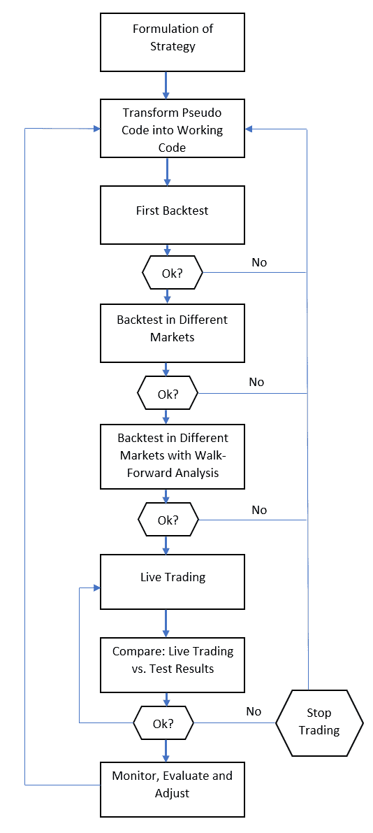
The walk-forward analysis is the most crucial building block of your trading strategy. At this stage it is determined if the hypothetical returns are a result of overfitting or the result of a robust trading system. If the walk-forward analysis produces negative results you must go back to the first step of your strategy development process. The analysis answers three essential questions: is the trading system profitable, what is it the profit factor to be expected in real time trading and how will changes in market conditions affect my strategy performance.
Elements of a Trading Strategy
- Entry and exit rules
- Risk management
- Position sizing
The effective formula to analyze strategy risk is the maximum drawdown multiplied with a margin of safety. The safety multiplier should be around 1.5. The concept can be extended adding required capital for the strategy consisting of following elements: maximum drawdown, margin requirements and safety factor. For example let’s assume we are trading the E-MINI S&P 500 the account size required would be, $15,000 (maximum drawdown) multiplied with 1.5 and adding $13,100 (margin requirements), $35,600. However, this model is not taking the fact into account that we could hit our worst case scenario right at the beginning of our trading journey. This is the reason why we need to consider a more conservative approach: $15,000 (maximum drawdown) multiplied with 1.5 and adding 2 times $13,100 (margin requirements). In this scenario we can weather two extreme drawdowns and continue trading our strategy.
Manage Profit with Exit Orders
To manage profit means preservation of capital. The main goal is to capture as much profit as possible. There are several different methods to achieve this. Here is a brief explanation of the more popular order types you can use.
Auction: An Auction order is entered into the electronic trading system during the pre-market opening period for execution at the Calculated Opening Price (COP).
Discretionary: An Discretionary order is a limit order submitted with a hidden, specified ‘discretionary’ amount off the limit price which may be used to increase the price range over which the limit order is eligible to execute. The market sees only the limit price.
Market: A Market order is an order to buy or sell at the market bid or offer price.
Market If Touched: A Market If Touched (MIT) is an order to buy (or sell) a contract below (or above) the market. Its purpose is to take advantage of sudden or unexpected changes in share or other prices and provides investors with a trigger price to set an order in motion.
Pegged To Market: A pegged-to-market order is designed to maintain a purchase price relative to the national best offer (NBO) or a sale price relative to the national best bid (NBB). Depending on the width of the quote, this order may be passive or aggressive.
Pegged To Stock: A Pegged to Stock order continually adjusts the option order price by the product of a signed user-define delta and the change of the option’s underlying stock price. The delta is entered as an absolute and assumed to be positive for calls and negative for puts. A buy or sell call order price is determined by adding the delta times a change in an underlying stock price to a specified starting price for the call.
Pegged To Primary: Relative (a.k.a. Pegged-to-Primary) orders provide a means for traders to seek a more aggressive price than the National Best Bid and Offer (NBBO). By acting as liquidity providers, and placing more aggressive bids and offers than the current best bids and offers, traders increase their odds of filling their order. Quotes are automatically adjusted as the markets move, to remain aggressive. For a buy order, your bid is pegged to the NBB by a more aggressive offset, and if the NBB moves up, your bid will also move up. If the NBB moves down, there will be no adjustment because your bid will become even more aggressive and execute. For sales, your offer is pegged to the NBO by a more aggressive offset, and if the NBO moves down, your offer will also move down. If the NBO moves up, there will be no adjustment because your offer will become more aggressive and execute.
Sweep To Fill: Sweep-to-fill orders are useful when a trader values speed of execution over price. A sweep-to-fill order identifies the best price and the exact quantity offered/available at that price, and transmits the corresponding portion of your order for immediate execution.
Limit Order: A Limit order is an order to buy or sell at a specified price or better. The Limit order ensures that if the order fills, it will not fill at a price less favorable than your limit price, but it does not guarantee a fill.
Box Top: A Box Top order executes as a market order at the current best price. If the order is only partially filled, the remainder is submitted as a limit order with the limit price equal to the price at which the filled portion of the order executed.
Limit If Touched: A Limit if Touched is an order to buy (or sell) a contract at a specified price or better, below (or above) the market. This order is held in the system until the trigger price is touched. An LIT order is similar to a stop limit order, except that an LIT sell order is placed above the current market price, and a stop limit sell order is placed below.
Limit On Close: A Limit-on-close (LOC) order will be submitted at the close and will execute if the closing price is at or better than the submitted limit price.
Limit On Open: A Limit-on-Open (LOO) order combines a limit order with the OPG time in force to create an order that is submitted at the market’s open, and that will only execute at the specified limit price or better. Orders are filled in accordance with specific exchange rules.
Passive Relative: Passive Relative orders provide a means for traders to seek a less aggressive price than the National Best Bid and Offer (NBBO) while keeping the order pegged to the best bid (for a buy) or ask (for a sell). The order price is automatically adjusted as the markets move to keep the order less aggressive. For a buy order, your order price is pegged to the NBB by a less aggressive offset, and if the NBB moves up, your bid will also move up. If the NBB moves down, there will be no adjustment because your bid will become aggressive and execute. For a sell order, your price is pegged to the NBO by a less aggressive offset, and if the NBO moves down, your offer will also move down. If the NBO moves up, there will be no adjustment because your offer will become aggressive and execute. In addition to the offset, you can define an absolute cap, which works like a limit price, and will prevent your order from being executed above or below a specified level. The Passive Relative order is similar to the Relative/Pegged-to-Primary order, except that the Passive relative subtracts the offset from the bid and the Relative adds the offset to the bid.
Stop: A Stop order is an instruction to submit a buy or sell market order if and when the user-specified stop trigger price is attained or penetrated. A Stop order is not guaranteed a specific execution price and may execute significantly away from its stop price. A Sell Stop order is always placed below the current market price and is typically used to limit a loss or protect a profit on a long stock position. A Buy Stop order is always placed above the current market price. It is typically used to limit a loss or help protect a profit on a short sale.
Stop Limit: A Stop-Limit order is an instruction to submit a buy or sell limit order when the user-specified stop trigger price is attained or penetrated. The order has two basic components: the stop price and the limit price. When a trade has occurred at or through the stop price, the order becomes executable and enters the market as a limit order, which is an order to buy or sell at a specified price or better.
Trailing Stop: A sell trailing stop order sets the stop price at a fixed amount below the market price with an attached “trailing” amount. As the market price rises, the stop price rises by the trail amount, but if the stock price falls, the stop loss price doesn’t change, and a market order is submitted when the stop price is hit. This technique is designed to allow an investor to specify a limit on the maximum possible loss, without setting a limit on the maximum possible gain. “Buy” trailing stop orders are the mirror image of sell trailing stop orders, and are most appropriate for use in falling markets.
Profit Target
Another method to protect your profits is to take a price level at which you will exit the trade. Using a profit target is a more aggressive way to lock in profits. The negative twist to this approach is that you might exit your trades too early.
Generally speaking profit targets produce a higher percentage of winning trades and a smoother equity curve. Overall performance can become more stable and usually such a method can be used when designing high frequency trading systems. On the contrary trend following strategies benefit the least from profit targets.
The profit target order is entered as a limit order and GTC. Overnight price change can influence the price level of the sell price order and it will be filled at the opening price. Basically this means when holding the position overnight in case of a opening gap we get a fill price X points higher than the price level of our sell price order. Systems that have tight profit targets are especially vulnerable to overnight gaps.
Position Size
The trading size determines our bet size and represents a crucial component of our trading system. Sizing rules have huge impact on our overall portfolio performance. However, efficient position sizing is difficult. One of the problems with effective position sizing arises from fat-tailed distributions that can severely impact our results.
If you want to make an impression at a board meeting employ the figure of speech now sweeping the economic world: “But what about the fat tail?” This is another way of asking “How come all you geniuses didn’t realize the risk you were running?” Embarrassed witnesses and recently fired C.E.O.’s explain that the distribution of values and risks long beloved by managers, credit-rating agencies and securities analysts turned out to be not so normal after all.
William Safire. Fat Tail. The New York Times Magazine.
Another problem is the lack of statistical robustness of many measures when applied to position sizing. It is important to be aware that position sizing can break or make a trading system.
Next we discuss four different position sizing models that you can implement in your strategy:
- Kelly Method
- Volatility Method
- Martingale
- Anti-Martingale
Here is an example, the following formula is derived from the Kelly method which was applied by Professor Edward Thorpe to gambling and trading.
Kelly% = (Win% – Loss%) / (Average Profit / Average Loss)
Assuming that a strategy has a winning percentage of 60%, an average win of $3000 and average loss of $1500, the Kelly % will tell us the % of our trading capital to risk on our next trade.
- Kelly% = (60 – 40) / ($3000 / $1500)
- Kelly% = 10%
Next we calculate our position size. We have our risk size being 10% of our equity. A risk per contract of $1000 and an account size of $500,000. The trade size is calculated as follows:
- Total Equity to Risk = $500,000 x 0.1
- Total Equity to Risk = $50,000
- Number of Contracts = $50,000 / $1,000
- Number of Contracts = 50
Please notice that these numbers often lack statistical robustness and should be used as a guide rather than an exact number.
The Volatility Method determines your position size according to current market volatility. A popular approach is using the ATR. Here is the formula of a 2 x ATR stop:
Position Size = ((porfolio size * % of capital to risk)/(ATR*2))
Example:
- Account value $300,000
- ATR of traded asset $15
- Asset trades at $290
Let’s assume you are willing to lose 5% of your capital on each trade, equivalent to $15,000 in our example. You also have to decide how many ATR units you are willing to let the asset go against you before you exit your position. In our formula we went for a 2 x ATR stop.
Using our risk parameters, we are willing to exit our position if we lose 6%. We get this percentage number by multiplying a 20 period ATR of our asset by our risk parameter of a 2 x ATR stop. We now have the absolute value of our stop, which is $30. We divide our 5% risk capital ($15,000) by $30 and we get the number of units to buy. In this example 500.
Calculate ATR: TR value is simply the High minus the Low, and the first 20-day ATR is the average of the daily TR values for the last 20 days.
Another approach to volatility based position sizing is the cluster volatility method, which can be applied to the S&P 500. We calculate the volatility of the S&P 500 for each cluster depending on the VIX level. So for example, a VIX price of 15-17 represents one cluster, 17.1-19 represents the second cluster; Each of these price intervals determines our risk size. In this scenario there is an upper limit to the maximum volatility stop depending on our strategy performance metrics.
The martingale method doubles the trade size after each loss and starts at one unit after each win. This method is derived from a gambling money management method. On the contrary the anti-martingale method starts with doubling the number of trade units after each win and starts at one after a loss.
Mind Opening and Closing Slippage
If your strategy is trading the opening price most databases include the first tick of the day or the midpoint of that opening range. For your backtesting results it means that your order is filled at market open. In reality a market order on the opening is filled within the opening range filled near the worst possible price. This form of slippage can add up if your strategy is executing a lot of trades and especially during market opening and within the last minutes of market close. As with the opening price the closing price in your database will be used as the price of the fill for the market on close order. The real execution price will be within the closing range.
Limit Move Circuit Breaker and Economic Events
Another issue considering your backtest results are limit moves. Futures contracts have daily trading limits which determine the maximum price fluctuation. In rare circumstances a market can open limit up or limit down and remain at this price level for the rest of the trading day. The limit move acts as a circuit breaker and is the maximum amount of change that the price of a commodity futures contract is allowed to undergo in a single day. This amount gets its basis from the previous day’s closing price. A trading strategy should not enter any trades on locked limit days. Reliable backtest results should exclude these types of days.
Major event trades should also be excluded from your strategy backtest except in those cases where you are running an event driven strategy. Most traders make it a practice not to enter trades within predetermined time bands around the release of key economic reports. During these events massive price slippage will occur. There are opposing views in the trading community on whether these trades should be included in your backtest results. Many argue that a well designed systematic strategy should be able to weather such event driven volatility storms successfully. In our view it depends on the strategy type you are running and your trading frequency.
Expiration and contract roll
Futures contracts have a limited lifespan that will influence the outcome of your trades and exit strategy. The two most important expiration terms are expiration and rollover.
A contract’s expiration date is the last day you can trade that contract. This typically occurs on the third Friday of the expiration month, but varies by contract.
Prior to expiration, a futures trader has three options:
- Rollover is when a trader moves his position from the front month contract to a another contract further in the future. Traders will determine when they need to move to the new contract by watching volume of both the expiring contract and next month contract. A trader who is going to roll their positions may choose to switch to the next month contract when volume has reached a certain level and the price difference between the two contracts is at the lowest level.
- Offsetting or liquidating a position is the simplest and most common method of exiting a trade. Usually when executing a high number of intraday trades, position rollover will be of a lesser concern.
- If a trader has not offset or rolled his position prior to contract expiration, the contract will expire and the trader will go to settlement.
When rolling the contract you have three options.
Unadjusted
The table below shows a theoretical futures contract. The first column counts the roll day. The next two shows the prices for February and March contracts.
| Day | Feb | March | Unadjsuted |
| -3 | 292 | 292 | |
| -2 | 293 | 293 | |
| -1 | 294 | 294 | |
| 0 | 295 | 300 | 300 |
| 1 | 301 | 301 | |
| 2 | 302 | 302 | |
The unadjusted columns as shown above do not adjust prices. On roll day we record the new prices for the February expiration. This method as seen on day 0 (rollover day) produces a price jump of $5. This price accurately reflect the price change but it distorts our backtest. Why? There is no way to capture that $5 profit.
Difference Adjusted
To remove these price differences between contract expiration’s we have to adjust our price. We have two choices here. We can start with a price in the past and adjust forward or we start with the current price and adjust back. Since it is helpful to have the current price match the current price of our series we will always back adjust. This means when adjusting a futures time series the prices that show up on our chart are not the prices the instrument traded at.
The first method to do this is to take the price difference between the new and old contracts and add that difference to old prices. Below table shows an example of this method.
| Day | Feb | March | Diff Adjusted |
| -3 | 292 | 297 | |
| -2 | 293 | 298 | |
| -1 | 294 | 299 | |
| 0 | 295 | 300 | 300 |
| 1 | 301 | 301 | |
| 2 | 302 | 302 | |
The above rollover method shows prices increasing by $1 and our time series has no price jump of $5. Now we have a back adjusted price of $299 prior to the roll day accurately reflecting the $1 price increase ($294 – $295).
Ratio adjusted
As shown the difference adjusted method preserves price changes for all historical prices in our times series. However, in order to preserve percent changes the ratio adjusted method must be used. Here are the steps to calculate it:
- Choose roll dates
- Start at current price and work backwards creating a variable called roll differential. For rollover days the roll differential is contract price/old contract price.
- Create variable cumulative roll differential, set to 1. Work backwards to calculate cumulative roll differential=tomorrow’s cumulative roll differential*today’s roll differential.
- Multiply fronth month price by roll differential.
Below shows the method applied.
| Jan | Feb | Mar | Roll Diff | Cum Diff | Ratio Adj. |
| 292 | 1 | 1.0344 | 301.75 | ||
| 293 | 1 | 1.0334 | 303.08 | ||
| 294 | 1 | 1.0334 | 303.82 | ||
| 295 | 300 | 1.0169 | 1.0165 | 304.95 | |
| 301 | 1 | 1.0165 | 305.96 | ||
| 302 | 1 | 1.0165 | 306.98 | ||
| 303 | 308 | 1.0165 | 1.00 | 308 | |
| 309 | 1 | 1.00 | 309 | ||
| 310 | 1 | 1.00 | 310 | ||
| 311 | 1 | 1.00 | 311 |
Most data vendors use difference adjusted time series data. They preserve point values of each swing but percent changes are seriously distorted. Ratio adjusted charts keep the percent changes but not the point values. These comes with issues for system developers.
If your system counts tick changes then you must implement the difference adjusted rollover method. On the other side if you calculate your system performance P&L as percentage of returns you must use a the ratio adjusted method.
When backtesting your strategy you must use a back adjustment method. You can model the actual rolls but you still need to decide how to calculate your entry signals. One of the more prominent data vendors (tickdata) recommends the following “Contract” and “Roll Method” settings for each futures symbol – see list.
Historical Data Backtesting Period
When deciding the time window to test a system there are two main considerations that must be satisfied, statistical soundness and relevance to the trading strategy. These requirements specify guidelines that can be followed to find the correct window size for a trading strategy.
Standard error is a mathematical concept used in statistics. In our case we can use this concept to give us insight on the required trade sample size. A large standard error indicates that the data points are far from the average and vice versa for a small standard error. Small standard error indicates a small variation of an individual winning trade from the average winning trade.
Standard Error = Standard Deviation/Square Root of the Sample Size
Next, we calculate three standard errors of the average winning trade on three different numbers of trades. The values used are:
- AVGw= avg. win
- StDev= standard deviation
- SqRT= square root
- Nw= number of winning trades
- Standard Error = StDev(AVGw)/SqRT(Nw)
The standard error measures the reliability of our average win as a function of the number of winning trades. Within the range we opt for the conservative assumption, the lower band of the average win. For example, with an average win of $400 and a standard error of $100 a typical win will be within the range of $300 to $500. In case of different trade sample sizes we can consider three examples of standard error based on trade sample sizes of 30, 90 and 300. We assume a standard deviation of our winning trades to be $200.
When our number of wins is 30 the standard error is:
Standard Error = 200/SqRT(30) -> 200/5.47722 = 36.51
A trade sample size of 30 gives us a standard error of $36.51. Which means our range of wins is $400 +/- $36.51. In a trade sample size of 90 winning trades the standard error is $21.09. In this case we have a range of $378.9 – $421.09. With a sample size of 300 we get wins that are in the range of $200 +/- $11.54.
Therefore the larger the sample size the lower the standard error of variance of winning trades. Based on this information we can conclude that more trades are better. Unfortunately, we do not always have a large trade sample size. This means when testing a strategy that has less frequent trades, we have to make the trade window as large as possible. Market practitioners seem fond of the number 30 as the smallest sample size that can be evaluated.
Additionally, trades should be evenly distributed throughout the backtest window. A small standard deviation of size and length of wins and losses increases the probability of a more robust trading strategy.
From Idea and Code to Preliminary Testing
The test results must now be evaluated and compared to theoretical expectations. We must analyze if our preliminary testing results are in line with the theoretical foundation. Which means that our first simulation should be in line with the assumed behavior of our system. Keep in mind that these are just rough expectations. If our results deviate dramatically from the theoretical foundation we must find the cause for it. If the strategy seems to be flawed we must redesign keeping our theoretical expectations in mind. At this stage it is important to rule out unusual market activity as the cause, as we have explained earlier – limit move circuit breaker and economic events.
When all the stars are aligned after reworking our idea and the strategy performance seems to be more consistent, we can move to the next step. At this point we have checked the following parameters: formulas calculated correctly, trading rules perform as programmed and results are consistent with theoretical expectation.
Performance Check
Next we estimate the profitability. First we calculate profit and loss for a current length of price history. Short term strategies can be tested on one to two years of data, intermediate term strategies on two to four years and long term strategies on four to eight years. These are guidelines with possible variances in the given time windows. Since we are in the beginning phase of our testing the performance of the strategy should at least be mildly profitable. A high unusual loss should be considered a preliminary warning sign. If this large loss occurred under “normal” market conditions we should consider going back to the drawing board.
Multi Market and Multi-Time Frame Test
Several historical simulations are produced. The purpose is to obtain a quick idea how robust the trading system is. This testing round is not conclusive but can provide valuable insight into the in and outs of the strategy. If the strategy performs well across several different markets it is a strong indication of a robust system. On the contrary a strategy performing poorly among many different markets and time frames is a sign that the strategy should be abandoned. Of course these tests assume that you are designing a strategy that is supposed to trade across several different markets. If you are working on just a specific market this test can be skipped.
If the strategy trades several different markets it is best to select a basket of uncorrelated markets. There are two criteria that provide a measure of the degree of difference between markets: correlation and fundamental diversity. For example coffee, corn and T-bonds are governed by different fundamental conditions.
Next we decide on whether to segment the testing period or not. To segment the price history is a statistically sound decision. It creates a statistically significant sample of trades. A trading strategy with a 300% return within two years might be impressive at the first glance but what if the majority of the profit was generated within the firs five weeks of trading? Therefore it is better to divide the entire historical period into an equal number of smaller intervals.
At this stage we consider small profits and small losses randomly distributed through the different time segments as an acceptable performance at this stage. As already mentioned at this stage we are only determining if the strategy is worthy of further development.
Optimization Process
Optimization is also known as search function or objective function. Most applications use grid search functions to arrive at the optimal combination of parameters.
The search method and number of parameters to be optimized will determine the processing time to complete the optimization. There may not be enough processing resources to calculate all the possible combinations and so intelligence on the part of the search method is used to guide the search in the right direction. A successful completion of such a test should meet the minimum criteria such as net profit above zero and drawdown less than 20 percent.
Grid Search
This is the most basic search method. It is a brute force method that calculates and then ranks every backtest. Let’s consider a backtest with changing time intervals for our entry signal. We test 15 minute intervals over a range of 90 minutes into the trading day beginning at the market opening. Seven different values will be tested 15min, 30min, 45min,….., 150min (11am).
The second variable will test our exit signal in 15 minute intervals for 90 minutes from 11 am until 12:30 pm.
The test run consists of 49 possible combinations of these scan ranges. Each value is tested with the first potential value for the for our exit signal as follows:
| Entry Signal | 930 | 945 | 1000 | 1015 | 1030 | 1045 | 1100 | |||
| Exit Signal | 1100 | 1100 | 1100 | 1100 | 1100 | 1100 | 1100 |
After the test cycle is completed the second variable of our exit signal is tested.
| Entry Signal | 930 | 945 | 1000 | 1015 | 1030 | 1045 | 1100 | |||
| Exit Signal | 1115 | 1115 | 1115 | 1115 | 1115 | 1115 | 1115 |
This process is repeated until all possible combinations are tested. This method is known as the grid search.
Here is an example of a large grid search experiment using Python.
model = RandomForestRegressor(n_jobs=-1, random_state=42, verbose=2)

grid = {'n_estimators': [10, 13, 18, 25, 33, 45, 60, 81, 110, 148, 200],
        'max_features': [0.05, 0.07, 0.09, 0.11, 0.13, 0.15, 0.17, 0.19, 0.21, 0.23, 0.25],
        'min_samples_split': [2, 3, 5, 8, 13, 20, 32, 50, 80, 126, 200]}

rf_gridsearch = GridSearchCV(estimator=model, param_grid=grid, n_jobs=4,
        cv=cv, verbose=2, return_train_score=True)

rf_gridsearch.fit(X1, y1)

# after several hours
df_gridsearch = pd.DataFrame(rf_gridsearch.cv_results_)
You can run a randomized search to analyze only a subsample of the data or grid search to explore the full grid of parameters.
The advantage of the method is that every possible parameter is evaluated. The drawback is its speed. The processing time increases significantly for large data sets. Let’s assume you have four different variables with the following ranges:
| EV | 1-20 | steps of 2=10 |
| OB | 10-90 | steps of 10=9 |
| RT | 15-105 | steps of 10=9 |
| RT² | 200-350 | steps of 5=30 |
To calculate the total number of tests we have to multiply the number of steps (10 x 9 x 9 x 30 = 24,300). If one test takes 1 second this optimization run will take (24,300/60 sec.)/60min. = 6.75 hours. Note we have used large steps, when testing in smaller steps the amount of time it takes to complete a grid search would be considerably higher.
Once the optimization space exceeds two dimensions analyzing the results is nearly impossible. For tests running three and more dimensions we need to use a more sophisticated optimization algorithm.
Hill Climbing Algorithm
Hill climbing algorithm is a local search algorithm which continuously moves in the direction of increasing elevation/value to find the peak of the mountain or best solution to the problem. It terminates when it reaches a peak value where no neighbor has a higher value.
The effect of this selectivity is the ability to determine an optimal parameter set while examining only a small sample of the optimization space. The risk with this method is that it can suffer from a lack of thoroughness. The method can select the global maximum and miss the best parameter in the entire optimization space.
There are three types of hill climbing algorithms:
1. Algorithm for Simple Hill Climbing:
- Step 1: Evaluate the initial state, if it is goal state then return success and Stop.
- Step 2: Loop Until a solution is found or there is no new operator left to apply.
- Step 3: Select and apply an operator to the current state.
- Step 4: Check new state:
- If it is goal state, then return success and quit.
- Else if it is better than the current state then assign new state as a current state.
- Else if not better than the current state, then return to step2.
- Step 5: Exit.
2. Steepest-Ascent hill climbing:
The steepest-Ascent algorithm is a variation of simple hill climbing algorithm. This algorithm examines all the neighboring nodes of the current state and selects one neighbor node which is closest to the goal state. This algorithm consumes more time as it searches for multiple neighbors
Algorithm for Steepest-Ascent hill climbing:
- Step 1: Evaluate the initial state, if it is goal state then return success and stop, else make current state as initial state.
- Step 2: Loop until a solution is found or the current state does not change.
- Let SUCC be a state such that any successor of the current state will be better than it.
- For each operator that applies to the current state:
- Apply the new operator and generate a new state.
- Evaluate the new state.
- If it is goal state, then return it and quit, else compare it to the SUCC.
- If it is better than SUCC, then set new state as SUCC.
- If the SUCC is better than the current state, then set current state to SUCC.
- Step 5: Exit.
3. Stochastic hill climbing:
Stochastic hill climbing does not examine for all its neighbor before moving. Rather, this search algorithm selects one neighbor node at random and decides whether to choose it as a current state or examine another state.
Hill climbing search Python implementation:
import math

increment = 0.1
startingPoint = [1, 1]
point1 = [1,5]
point2 = [6,4]
point3 = [5,2]
point4 = [2,1]

def distance(x1, y1, x2, y2):
    dist = math.pow(x2-x1, 2) + math.pow(y2-y1, 2)
    return dist

def sumOfDistances(x1, y1, px1, py1, px2, py2, px3, py3, px4, py4):
    d1 = distance(x1, y1, px1, py1)
    d2 = distance(x1, y1, px2, py2)
    d3 = distance(x1, y1, px3, py3)
    d4 = distance(x1, y1, px4, py4)

    return d1 + d2 + d3 + d4

def newDistance(x1, y1, point1, point2, point3, point4):
    d1 = [x1, y1]
    d1temp = sumOfDistances(x1, y1, point1[0],point1[1], point2[0],point2[1],
                                point3[0],point3[1], point4[0],point4[1] )
    d1.append(d1temp)
    return d1

minDistance = sumOfDistances(startingPoint[0], startingPoint[1], point1[0],point1[1], point2[0],point2[1],
                                point3[0],point3[1], point4[0],point4[1] )
flag = True

def newPoints(minimum, d1, d2, d3, d4):
    if d1[2] == minimum:
        return [d1[0], d1[1]]
    elif d2[2] == minimum:
        return [d2[0], d2[1]]
    elif d3[2] == minimum:
        return [d3[0], d3[1]]
    elif d4[2] == minimum:
        return [d4[0], d4[1]]

i = 1
while flag:
    d1 = newDistance(startingPoint[0]+increment, startingPoint[1], point1, point2, point3, point4)
    d2 = newDistance(startingPoint[0]-increment, startingPoint[1], point1, point2, point3, point4)
    d3 = newDistance(startingPoint[0], startingPoint[1]+increment, point1, point2, point3, point4)
    d4 = newDistance(startingPoint[0], startingPoint[1]-increment, point1, point2, point3, point4)
    print i,' ', round(startingPoint[0], 2), round(startingPoint[1], 2)
    minimum = min(d1[2], d2[2], d3[2], d4[2])
    if minimum < minDistance:
        startingPoint = newPoints(minimum, d1, d2, d3, d4)
        minDistance = minimum
        #print i,' ', round(startingPoint[0], 2), round(startingPoint[1], 2)
        i+=1
    else:
        flag = False
It’s important to note that a hill-climbing algorithm which never makes a move towards a lower value is guaranteed to be incomplete because it can get stuck on a local maximum. And if the algorithm applies a random walk, by moving a successor, then it may complete but not efficient. Simulated Annealing is an algorithm which yields both efficiency and completeness.
Simulated Annealing
Simulated Annealing (SA) is an effective and general form of optimization. It is useful in finding global optima in the presence of large numbers of local optima. “Annealing” refers to an analogy with thermodynamics, specifically with the way that metals cool and anneal. Simulated annealing uses the objective function of an optimization problem instead of the energy of a material.
Implementation of SA is surprisingly simple. The algorithm is basically hill-climbing except instead of picking the best move, it picks a random move. If the selected move improves the solution, then it is always accepted. Otherwise, the algorithm makes the move anyway with some probability less than 1. The probability decreases exponentially with the “badness” of the move, which is the amount deltaE by which the solution is worsened.
For more information on this algorithm and how to implement it read Simulated annealing algorithm for optimal capital growth or Simulated annealing for complex portfolio selection problems.
Genetic Algorithms
These kind of algorithms mimic the biological process of evolution. They are robust and fast using the process of mutation to reduce the likelihood of getting stuck on a local optimum. Below you can see a simplified overview of how the algorithm operates.
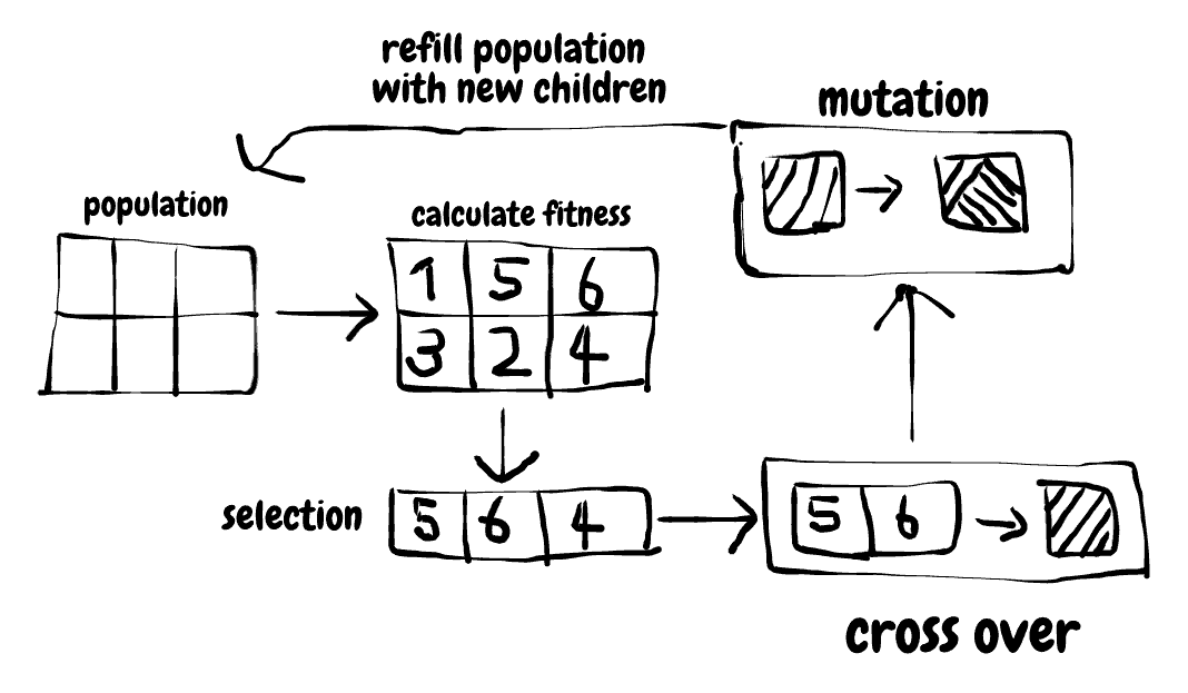
Since the optimization space of a trading strategy can be complex the efficiency of a genetic algorithm recommends them for strategy development.
The algorithm proceeds with repeating the steps for successive generations. Each generation produces a new population of parameter sets. This process continues until:
- Predetermined number of generations have been evaluated.
- A good solution has been found.
- Significant improvement in the fitness of the population is no longer made.
Genetic search methods tend to find a good solution but do not guarantee to find the best possible solution. However, it should be close to the best possible solution. The algorithm can identify top parameters by evaluating only 5 to 10 percent of the total candidate population.
Here is a simple implementation of a genetic algorithm using Python:
i=0
fitness = 0
counter = 0
while i < max_iter:
   if counter > n_repeats:
      STOP
   Y = [ ]
   fit = [ ]
   pairs = randompairsfrom (X)
   for j in pairs:
      y = crossover ( j )
      y = randommutation ( y )
      Y. append (y)
      fit.append (fitness(y))
   Y, fit = ordermaxtomin (Y, fit )
   bestfitness = fit[ 0 ]
   if bestfitness < fitness:
      counter = counter+1
   else:
      counter = 0
      X = Y [0: N]
      i=i+1
      fitness = bestfitness
For a more complex example read Generating Long-Term Trading System Rules Using a Genetic Algorithm Based on Analyzing Historical Data.
Particle Swarm Optimization
Particle swarm optimization begins with selecting a group of potential strategy parameters located randomly throughout the optimization space. A positive or negative velocity is also assigned by chance determining the speed at which the parameter set is adjusted. To visualize it, imagine the parameter as a particle flying through the optimization space.
The same parameter sets persist throughout the optimization process but their positions in the optimization space change continuously. In the next step during each iteration of the PSO, each parameter set is adjusted in its position. Third, each particle remembers its personal best location in the optimization space. Fourth, each particle also updates the other particles when it finds a new global best spot.
Like with genetic algorithms the effective application of a PSO relies heavily on the quality of the search function.
Limitations
Since direct search methods do not evaluate every possible parameter set combination, there is a certain degree of uncertainty included in the backtest results. They are not able to find the global maxima. Many of these search methods will encounter problems when searching a spiky optimization space.
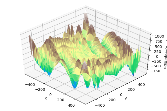
If your optimization set looks the same as the graph shown above you should seriously consider reworking your idea. The application of any search method will not produce reliable parameter results in the case of a spiky optimization space.
The best evaluation method is the one which will select the parameter set for a trading strategy that is most predictive of real-time trading success. In order to evaluate the method used the key characteristics of a good trading strategy must consist of:
- Even distribution of trades
- Even distribution of trading profits
- Long/Short profit balanced
- Large group of profitable strategy parameters in the optimization
- Risk parameter acceptable/stress test/largest drawdown
- Balanced winning and losing runs
- Large number of trades
Evaluate strategy performance
For the evaluation of a strategy we use a more advanced method which is a correlation between equity curve and perfect profit. It measures the strategy performance to the actual profit potential provided by the market. In this context perfect profit represents a theoretical measure of market potential. It is the total profit of selling every peak and buying every trough.
The equity curve is the sum of the beginning account balance, closed trades and open trade profit. The correlation between equity curve and perfect profit is the correlation coefficient between the two which ranges from -1 to +1. A value close to +1 suggests a good trading strategy as it tells us that the equity curve is rising in tandem with the perfect profit. Here is the formula:
Correlation Coefficient = Sum [(x(i) – M’x)(y(i) – M’y)/[(n – 1) x SD’x x SD’y]
- n = number of days
- x = perfect profit
- y = equity curve
- M’x = mean of perfect profit
- M’y = mean of equity curve
- SD’x = standard deviation of perfect profit
- SD’y = standard deviation of equity curve
The closer the correlation to +1 the more effective the strategy is capturing market opportunities. Another key signal for a good strategy is that during periods of low volatility the strategy performance decreases but there is no large dip in the equity curve.
Another evaluation measure is called the pessimistic return on margin. It is an annualized yield on margin that assumes a strategy will perform less optimal during live trading than it did in historical backtests.
The gross profit is adjusted by calculating an adjusted lower gross profit. First we calculate the number of winning trades reduced by its square root. We are adjusting the strategy performance by its standard error. This number is than multiplied by the average winning trade and we get our adjusted lower gross profit. Next the gross loss is adjusted and we increase the number of losing trades by its square root. A new adjusted gross profit/loss is then calculated. This is used to produce an annualized rate of return on margin:
PROM = {[AW × (#WT − Sq(#WT))] − [AL × (#LT − Sq(#LT))]}/Margin
#WT = Number of Wins
AW = Average Win
#LT = Number of Losses
AL = Average Loss
A#WT = Adjusted Number of Wins
A#LT = Adjusted Number of Losses
AAGP = Adjusted Annualized Gross Profit
AAGL = Adjusted Annualized Gross Loss
A#WT = #WT − Sq(#WT)
A#LT = #LT + Sq(#LT)
AAGP = A#WT × AW
AAGL = A#LT × AL
Here is an example:
- $150,000 annualized gross profit
- 67 wins
- $40,000 annualized gross loss
- 28 losses
- A margin of $30,000
The annualized rate of return on margin would be 367%. [$150,000 – $40,000] / $30,000 = 3.667 = 367%
Calculating our return with the PROM formula:
Adjusted Number of Wins = 67 − Sq(67) = 58
Adjusted Number of Losses = 28 + Sq(28) = 34
Adjusted Annual Gross Profit = ($150,000/67) × 58 = $129,850
Adjusted Annual Gross Loss = ($40,000/28) × 34 = $48,571
PROM = ($129,850 − $48,571)/$30,000 = 2.7093
PROM = 271% per year
This calculation assumes that a trading system will never win as frequently in live trading as it did in the backtests. It reflects a pessimistic assumption and as such represents a more conservative measure. Additionally the measure penalizes small trade samples. The smaller the number of trades the more pessimistic profit and loss are adjusted. You can also add a more stringent derivative of the above formula by removing your largest winning trade from the gross profit.
Maximum Drawdown
Maximum drawdown plays an important role in the assessment of our strategy. There are many other measures of drawdown and it is helpful to look at them in relation to the maximum drawdown. In this context it is useful to know the average drawdown and minimum drawdowns. If the maximum drawdown is three times larger than the average drawdown it is a cause for further investigation. It is important to understand the market conditions that caused this drawdown. In some cases the large drawdown might be caused by unexpected events. This is why we cannot emphasize enough the importance of fat tails and how large of an impact it can have on your portfolio performance. Risk is one of the major costs in trading. Many investors don’t appreciate how ‘fat’ these tail risks are.
Optimization Framework
There are four key decision to be made to set up the framework:
- Variables and scan ranges that are to be used in the optimization must be defined
- Adequate data sample must be selected
- The search function that identifies the best parameters must be selected
- Guidelines for the evaluation of the optimization must be set
Variables
It is better to go for a smaller number of variables to avoid overfitting. Key strategy variables have to be identified which will be used for the optimization. The key variables are the ones that have the most significant impact on strategy performance. All other variables are to be excluded from the optimization process. If the significance of the variables is not known an added empirical step must be performed. The most effective way is to scan each variable separately, one at a time.
Scan Range and Step Size
There are two considerations to be made when defining the data range for our optimization. First the theoretical consideration, if we have short term trading strategy scanning a variable in a range from 1 to 1000 trading days doesn’t make sense. Why would you evaluate an intraday trading strategy that trades several times a day with data going back as far as 1000 trading days? A more appropriate parameter range would be 20 to 30 days.
Next we consider practical considerations. When scanning over large historical samples with multiple variables to optimize processing power becomes a real consideration. Remember our example with the steps in our calculation and the number of variables equals the total number of historical simulations. However, when testing with multiple variables it is best to keep the step sizes of each variable to be scanned proportional to one another. So for example, if the first variable range is 10 to 30 (10 x 3) at steps of 1 and the second variable starts at 40, then to keep this in proportion its range should end at ( 30 x 3) 90 and the step size should be 3. It is not always easy to find the best step sizes especially in multi- dimensional optimization environments. Nevertheless, it is important to attempt to arrive at the appropriate number of step sizes for each variable and to keep them in proportion to each other.
Historical Data
One of the most important parts of the optimization process is the size of the historical data. There are two main principles that define the data sample to be used:
- Large enough sample to produce statistically meaningful results
- Enough data to include different market conditions
As we have mentioned before you should have at least 30 trades. In practice you should have a much larger sample of trades. The second principle can prove to be more difficult to implement. The historical data sample should contain as many types of trends as possible. It should contain at least two of the four market trends: Congested, Cyclic, Bullish and Bearish. The data should also include a wide range of volatility levels.
It can be stated that that a robust and consistent trading strategy is defined by following attributes:
- Generating alpha on a broad possible range of parameter sets
- Across different market trends
- In a majority of different historical time periods
- Different volatility regimes and unexpected events – fat tailed distributions
Optimization Profile
There are three components that define the robustness of an optimization profile:
- Significant proportion of profitable variable sets within the total optimization universe.
- Distribution of performance throughout optimization space is evenly distributed with small variations.
- Shape of profitable variable sets. No large data jumps. More spiky or discontinuous shape of the optimization profile, the less likely it is that it is a robust trading strategy.
The greater the number of variable sets that produce profitable historical simulations the greater the likelihood that these results are statistically significant. Here are some examples of different optimization profiles:
| Number | Percentage | Average | |
| Number of Tests | 500 | 100% | $8,457 |
| Profitable Tests | 55 | 11% | $25,894 |
| Losing Tests | 445 | 89% | $8,415 |
| Number | Percentage | Average | |
| Number of Tests | 500 | 100% | $6,457 |
| Profitable Tests | 110 | 22% | $26,594 |
| Losing Tests | 390 | 78% | $3,815 |
| Number | Percentage | Average | |
| Number of Tests | 500 | 100% | $6,457 |
| Profitable Tests | 335 | 67% | $14,594 |
| Losing Tests | 165 | 33% | $2,115 |
If the optimization profile has passed the test of statistical significance we can next review the distribution within the total universe of variable sets. A robust trading strategy will have an optimization profile with a large average profit, small range between profit/loss and a small standard deviation.
Additional insights on the robustness of the optimization profile are given by:
- Optimal strategy variables performance is close to the average performance – within one standard deviation
- The average simulation results minus one standard deviation generates alpha
Shape of optimization profile
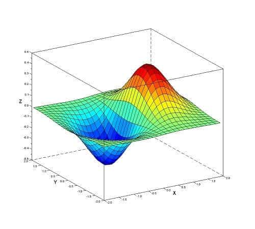
The above chart is an example of a variable set resting on top of a round and gradually declining hilltop of other profitable variable sets. It represents a solid optimization profile.
After evaluating the robustness of our strategy we must evaluate whether or not the strategy responded positively to our optimization process. In our final step the trading system must be put to the decisive test: Walk Forward Analysis.
Walk-Forward Analysis
The walk forward analysis judges the robustness of a system exclusively on the basis of out of sample trading. If the strategy performs well in this analysis it has shown to produce real world results and can be traded in real time. The analysis gives us answers to four questions:
- Is the system robust and can it generate alpha in real time trading?
- What rate of return is to be expected?
- How will changes in market behaviour affect strategy performance?
- What is the best variable set to use in real time trading?
The primary end goal is to evaluate whether the strategy is a robust process that can be repeated or rather the result of overfitting. Therefore the Walk-Forward Analysis is the only way to arrive at a statistically reliable measure of trading performance. Past research has shown that strategies that have 50 to 60 percent Walk-Forward Efficiency can be considered robust. On the contrary a poor strategy will not pass the WFA.
To achieve statistical validity during the WFA several walk-forwards must be performed on a trading strategy. If the results are consistent and in sample performance is close to out of sample performance we can conclude to have developed a very robust system.
Changing Market Conditions
There are seasonal tendencies across many markets especially in the agricultural markets. All markets go through cycles of peak and trough affected by contracting and expanding patterns of supply and demand. Markets can have periods of low and high volatility. Markets that are highly mean reverting offer price swings and also periods that have a strong trend. The fact that volatility changes continuously adds a significant amount of complexity to market patterns.
The discussion makes clear that a market can shift in many ways which makes the walk-forward analysis even more crucial for the design of a robust trading strategy.
The size of the in- and out-of-sample windows will depend on the trade frequency. Let us assume we are evaluating a short term trading system and that we have 1 year of tick data. The strategy is optimized on 9 months of tick data and a walk forward analysis is done on 3 months of data. The best variable set is tested on the 3 months of data. If more data is available we can do several WFA for data prior to the out of sample data set.
At this stage there are three main conclusions:
- If strategy loses money in majority of these walk-forward tests we do not have a tradable trading strategy.
- If strategy performs moderately on these tests it may be an argument for a poor to overfit strategy.
- If the strategy performs with out-of-sample profit in proportion to its in-sample profit in the majority of tests we can assume to have a robust trading strategy.
Following components are required for the walk-forward analysis:
- Scan ranges for variables
- Search function to be used
- Size of the optimization universe
- Size of in- and out-of-sample window
The size of the optimization universe is determined by:
- Trade frequency
- Style of trading strategy – momentum, trend, pattern recognition, event trading;
- Shelf life of trading variables
As mentioned before short term strategies benefit from shorter optimization windows from one to two years. Typically a walk forward window should be in the range of 25 to 35 percent of the optimization universe. When it comes to live trading a strategy that is optimized on two years of data will most likely remain stable for up to six months. A model built on 4 years of data will remain usable for one year and in the best case scenario for two years.
To illustrate consider the following example of a 2-variable scan on a 48-month optimization window.
| Asset | S&P 500 Futures |
| Optimization Size | 48 months |
| Price History | 03/27/2017 – 03/27/2020 |
| Buy Variable | Scan 0 to 150 in steps of 10 |
| Sell Variable | Scan 0 to 150 in steps of 10 |
In the first step we are optimizing two key variables from 03/27/2017 – 03/27/2020 on a variable space encompassing 256 candidates. After our test is completed we will have our top variable set.
In the next step our walk-forward analysis will determine the performance of our top variable set. New pieces of historical data are added to the analysis. We evaluate our performance on this new out-of-sample data. The results look as follows:
| Asset | S&P 500 Futures |
| Trading Window | 6 months |
| Trading Window Tested | 03/28/2020 – 09/27/2020 |
| Price History | 03/27/2017 – 03/27/2020 |
| Optimization P&L | $980,480 |
| Annualized Optimization P&L | $245,120 |
| Trading P&L | $489,000 |
| Annualized Trading P&L | $978,000 |
| Walk-Forward Efficiency | 300% |
The walk-forward analysis is done on 6 month of price history immediately after the optimization window. Our top variable set made $980,480 during the 48-month optimization test. The top variable set made $489,000 during its six month out-of-sample test which is annualized $978,000. While these results are impressive they could still be a product of chance which is why its essential to conduct a series of walk-forward tests. This is the most reliable method of evaluating the robustness of our system. A large number of walk-forward tests will diminish the likelihood that our strategy performance is the result of random chance. Another purpose of the walk-forward analysis is to verify the optimization process as a whole.
An important question asked among practitioners is how often should the system be reevaluated. The answer to that depends on the optimization and walk-forward windows. If for example the walk-forward window is six months then the model must be reoptimized after six months of trading.
Risk Factor and Drawdown
As a general rule of thumb a trading strategy that produces drawdowns in real time trading that exceed optimization drawdowns by a wide margin may be showing signs of trouble. In this context a walk-forward maximum drawdown is an important measure to watch.
Required Capital
It is beyond the scope of this article to delve into all the mathematical procedures for calculating required capital seeking maximum returns while minimizing risk.
Therefore we will continue with our formula for the calculation of required capital when trading futures. At minimum a trading account requires an initial margin plus the dollar value equal to the maximum drawdown.
Required Capital =Margin + Risk (maximum drawdown)
To protect yourself from maximum drawdown some investors tend to use the maximum drawdown equal three times the current maximum drawdown.
For example:
- Required Capital = Margin +(MDD X Safety Factor)
- Margin = $10,000
- Maximum Drawdown = $5,000
- Safety Factor = 3
- Required Capital = $10,000 + ($5,000 x 3)
- Required Capital = $25,000
Considering the importance of risk in trading the reward to risk ratio is a statistic that provides an easy comparison of reward and risk. Here is the formula:
RRR = Net Profit/Maximum Drawdown
The bigger the risk to reward ratio the better. It implies that profit is increasing relative to the risk. In general the RRR should be three or better.
And finally after successfully completing all those steps as described in our article you can reap the rewards of your hard work.
If you like our article sign up here for more in-depth research [We publish trading strategies & research using R, Python and EasyLanguage]
References
Sinclair, E. (2013). Volatility Trading, 2nd Ed. John Wiley & Sons.
Tsay, R. (2010). Analysis of Financial Time Series, 3rd Ed. Wiley-Blackwell.
Robert Pardo. (2008). The Evaluation and Optimization of Trading Strategies, 2nd Ed. John Wiley & Sons.
Scherer, B. and Douglas, M. (2005). Introduction to Modern Portfolio Optimization. Springer.
This is fantastic. Thanks.
There appears to be an error in the PROM formula; it indicates LT – LT^0.5, but is applied as LT+ LT^0.5.
Thanks for reading!
P.S. The product of two integers with like signs is equal to the product of their absolute values. The product of two negative integers is positive.
Sorry, I don’t follow. I was referring to this line:
PROM = {[AW × (#WT − Sq(#WT))] − [AL × (#LT − Sq(#LT))]}/Margin
but later it is applied as
Adjusted Number of Losses = 28 + Sq(28) = 34
The latter seems correct; I believe there is a sign error in the former wrt LT.
Thanks again. Great read.