

An Introduction to Probabilistic Deep Learning Explained in Simple Terms
Deep learning is nothing else than probability. There are two principles involved in it, one is the maximum likelihood and the other one is Bayes. It is all about maximizing a likelihood function in order to find the probability distribution and parameters that best explain the data we are working with. Bayesian methods come into play where our network needs to say, “I am not sure”. It is at the crossing between deep learning architecture and Bayesian probability theory.
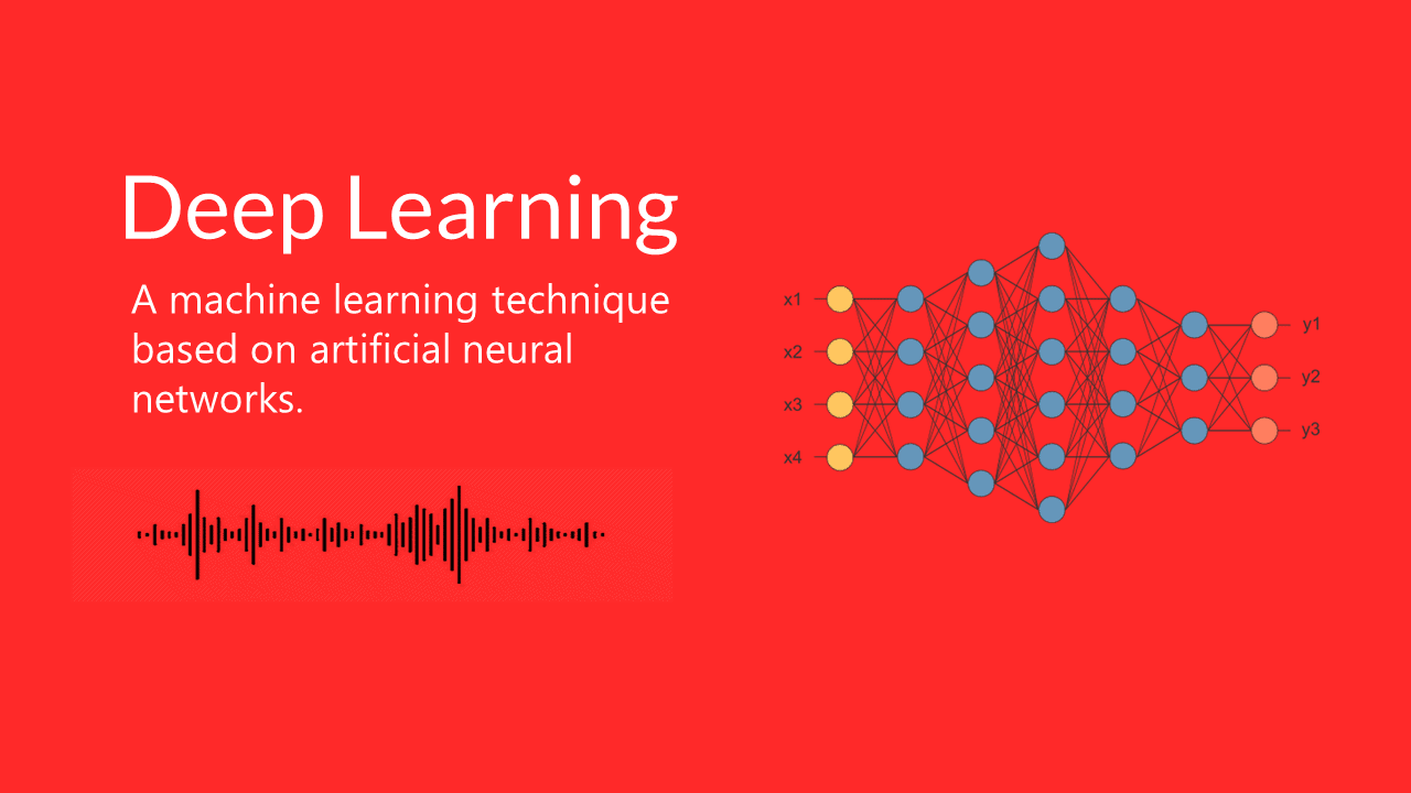
In general deep learning can be described as a machine learning technique based on artificial neural networks. To give you an idea of what an artificial neural network looks like see figure 1.
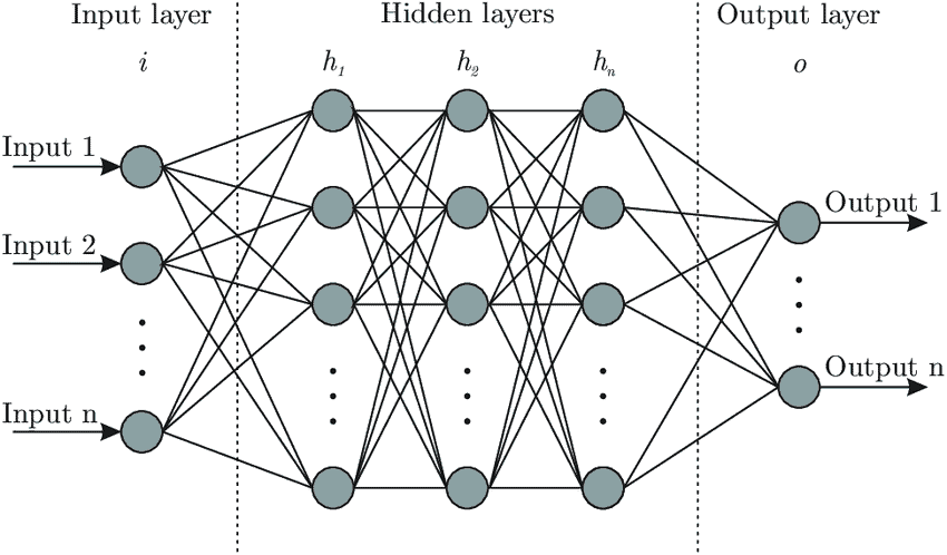
In figure 1 you can see an artificial NN with three hidden layers and several neurons on each layer. Each neuron is connected with each neuron in the next layer. The network simulates the way the human brain analyzes and processes information. While the human brain is quite complex, a neuron in an artificial NN is a simplification of its biological counterpart.
To get a better understanding imagine a neuron as a container for a number. The neurons in the input layer are holding the numbers. Such input data could be the historical volatility, and implied volatility of the S&P 500 Index. The neurons in the following layers get the weighted sum of the values from the connected neurons. The connections aren’t equally important, weights determine the influence of the incoming neuron’s value on the neuron’s value in the next layer. With the training data you tune the weights to optimally fit the data. Only after this step the model can be used for predictions.
Working with a deep learning system consists of two steps.
- Choosing the architecture for your given problem
- Tune the weights of the model
Classification
Classification involves predicting which class an item belongs to. Most classification models are parametric models, meaning the model has parameters that determine the course of the boundaries. The model can perform a classification after replacing the parameters by certain numbers. Tuning the weights is about how to find these numbers. The workflow can be summarized in three steps:
- Extracting features from the raw data
- Choosing a model
- Fitting classification model to the raw data by tuning the parameter
By using validation data you evaluate the performance of the model. It is similar to a walk forward analysis where you use the data set not used during the optimization of your parameters.
We differentiate between probabilistic and non-probabilistic classification models.
Probabilistic classification
It refers to a scenario where the model predicts a probability distribution over the classes. As an example from the stock market, a probabilistic classifier would take financial news and then output a certain probability of the stock market going up or down. Both probabilities add up to one. You would pick the trade with the highest probability.
However, if you provide the classifier with an input not relevant to the security the classifier has no other choice than assigning probabilities to the classes. You hope that the classifier shows its uncertainty by assigning more or less equal probabilities to the other possible but wrong classes. This is often not the case in probabilistic neural network models. This problem can be tackled if we extend the probabilistic models by taking a Bayesian approach.
Bayesian probabilistic classification
Bayesian Classification is a naturally probabilistic method that performs classification tasks based on the predicted class membership probabilities. Therefore Bayesian models can express uncertainty about their predictions. In our example above our model predicts the outcome distribution that consists of the probability for an up or down day. The probabilities add up to 1.
So, how certain is the model about the assigned probabilities? Bayesian models give us an answer to this question. The advantage of this model is that it can indicate a non reliable prediction by a large spread of the different sets of predictions.
Probabilistic deep learning with a maximum likelihood approach
To better understand this principle we start with a simple example far away from deep learning. Consider a die with one side showing a joker sign and the others displaying +/ -/ : / x / no sign /.
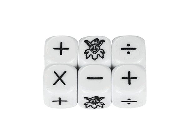
Now, what is the probability of the joker sign coming up if you throw the die? On average you get a joker sign one out of six cases. The probability is p= 1/6. The probability that it won’t happen is 1-p or 5/6. What is the probability if you throw the die six times? If we assume that the joker sign comes in the first throw and we see all the other signs in the next five throws, we could write this in a string as:
J*****
The probability for that sequence is 1/6 x 5/6 x 5/6 x 5/6 x 5/6 = 1/6 x (5/6)5 = 0.067 or with p= 1/6 as p1 x (1-p)6-1.
If we want the probability that a single joker sign and 5 other signs occur in the 6 throws regardless of the position, we have to take all the following 6 results into account:
J*****
*J****
**J***
***J**
****J*
*****J
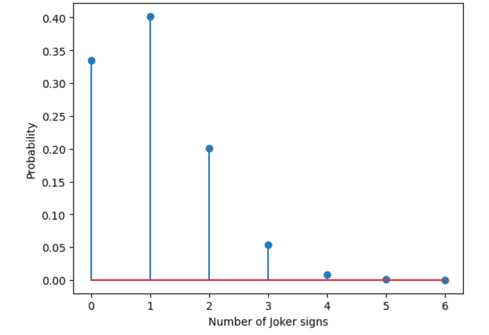
Each of these sequences has the same probability of p x (1-p)5. The probability that one joker sign occurs and any other sign five times is 0.067 or 6.7%. Calculating the probability for two joker signs in 6 throws we have 15 possible ways. The number 15 is derived from all permutations 6! divided by the number of indistinguishable permutations. This is 6! / (2! x 4!) = 15. The total probability of two joker signs and five * is 15 x (1/6)2 x (5/6)4 = 0.20.
The above example is called binomial experiment. The experiment has the following properties:
- The experiment consists of n repeated trials.
- Each trial can result in just two possible outcomes.
- The probability of success, denoted by p, is the same on every trial.
- The trials are independent, the outcome on one trial does not affect the outcome on another trial.
In the SciPy library we have a function called binom.pmf to calculate this with the arguments k equals the number of successes, n equals the number of tries, and p equals the probability for success in a single try. Below is the output for this experiment.
Below is the code for the experiment. You can run it on google colab.
try: #If running in colab
    import google.colab
    IN_COLAB = True
    %tensorflow_version 2.x
except:
    IN_COLAB = False

import tensorflow as tf
if (not tf.__version__.startswith('2')): #Checking if tf 2.0 is installed
    print('Please install tensorflow 2.0 to run this notebook')
print('Tensorflow version: ',tf.__version__, ' running in colab?: ', IN_COLAB)

#load required libraries:
import numpy as np
import matplotlib.pyplot as plt
%matplotlib inline
plt.style.use('default')

# Assume a die with only one face with a joker sign
# Calculate probability to observe in 6 throws 1- or 2-times the J-sign
6*(1/6)*(5/6)**5, 15*(1/6)**2*(5/6)**4

from scipy.stats import binom
# Define the numbers of possible successes (0 to 6)
njoker = np.asarray(np.linspace(0,6,7), dtype='int')
# Calculate probability to get the different number of possible successes
pjoker_sign = binom.pmf(k=njoker, n=6, p=1/6)
plt.stem(njoker, pjoker_sign)
plt.xlabel('Number of Joker signs')
plt.ylabel('Probability')
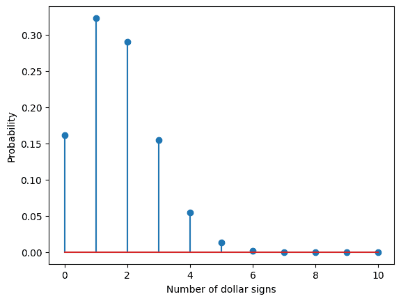
Now consider the following example, you are in a casino and play a game in which you win if a dollar sign appears. You know that there are a certain number of faces (0-6), but you don’t know how many. You observe 10 throws of a die with two dollar signs coming up in those throws. What do you think is the number of dollar signs on the die? By using the code above we can assume that our die this time has two faces with a dollar sign. Our observed data is fixed with ten throws and two dollar signs, but our model changes the data generated from a die with zero dollar faces to a die with 1,2,3…6 dollar faces. The probability of a dollar sign appearing is our parameter. The parameter takes the values p=1/6, 2/6…, 6/6 for our different models. The probability can be determined for each of the models. You can use the code below to calculate the probabilities for each of the models.
try: #If running in colab
    import google.colab
    IN_COLAB = True
    %tensorflow_version 2.x
except:
    IN_COLAB = False

import tensorflow as tf
if (not tf.__version__.startswith('2')): #Checking if tf 2.0 is installed
    print('Please install tensorflow 2.0 to run this notebook')
print('Tensorflow version: ',tf.__version__, ' running in colab?: ', IN_COLAB)

#load required libraries:
import numpy as np
import matplotlib.pyplot as plt
%matplotlib inline
plt.style.use('default')


# Assume a die with only one face with a dollar sign
# Calculate the probability to observe in 10 throws 1- or 2-times the $-sign
# See book section 4.1
10*(1/6)*(5/6)**9, 45*(1/6)**2*(5/6)**8

from scipy.stats import binom
# Define the numbers of possible successes (0 to 10)
ndollar = np.asarray(np.linspace(0,10,11), dtype='int')
# Calculate the probability to get the different number of possible successes
pdollar_sign = binom.pmf(k=ndollar, n=10, p=1/6)  #B
plt.stem(ndollar, pdollar_sign)
plt.xlabel('Number of dollar signs')
plt.ylabel('Probability')
#Solution for model assumption. Different number of dollar signs.
from scipy.stats import binom
#Define the considered numbers of dollar signs on the die (zero to six):
ndollar = np.asarray(np.linspace(0,6,7), dtype='int')
#Calculate corresponding probability of 2 $-signs in 10 throws
pdollar = binom.pmf(k=2, n=10, p=ndollar/6)
plt.stem(ndollar, pdollar)
plt.xlabel('Number of dollar signs on the dice')
plt.ylabel('Probability observing 2 dollar signs in 10 throws')
plt.title('Unnormalized likelihoods')
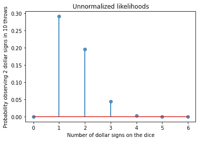
In our example the parametric model is the binomial distribution with two parameters. One parameter is p the probability and the other one is n the number of trials. For our model we chose the p value with the maximum likelihood, p= 1/6. The probabilities shown in the graph above are unnormalized in the sense they do not add up to 1. In the strictest sense they are not probabilities therefore we speak of likelihoods. The likelihoods can be used for ranking and to pick the model with the highest likelihood.
To summarize, for our maximum likelihood approach we need to do the following:
- We need a model for the probability distribution of the data that has one or more parameters. In our example the parameter is probability p.
- We use the model to determine the likelihood to get the observed data when assuming different parameter values.
- The parameter value is chosen for which the likelihood is maximal. This is called the Max-Like estimator. In our model the ML estimator is that the die has one side with a $-sign.
Loss functions for classification
Next, we discuss the use of the max-like principle to derive the loss function. In machine learning loss functions for classification are computationally feasible loss functions representing the price paid for inaccuracy of predictions in classification problems.
A loss function is useful when the true parameter is unknown. Typically we seek to minimize the error. In this context the objective function is often referred to as a loss function and the value calculated by this function is referred to as loss. To calculate the error of a model during optimization a loss function must be chosen.
Under the maximum likelihood principle the loss function estimates how closely the distribution of predictions made by a model matches the distribution of target variables in the training data. By using cross-entropy we measure the error between two probability distributions. With the maximum likelihood estimation we seek a set of model weights that minimizes the difference between the model’s predicted probability distribution given the time series data and the distribution of probabilities in the training set. We call this cross-entropy. Deep learning neural networks are trained using cross-entropy as the loss function in maximum likelihood frameworks.
What loss function to use under a framework of maximum likelihood?
The choice of a loss function is related to the activation function used in the output layer of our neural network. An activation function is a function that is added into an artificial neural network in order to help the network learn complex patterns in the data. When comparing with a neuron-based model that is in our brains, the activation function is at the end deciding what is to be fired to the next neuron.
Below is a short summary of best practice for each problem type with regard to the loss function.
Binary classification problem: This is the simplest kind of machine learning problem. The goal of binary classification is to categorize data points into one of two buckets: 0 or 1, true or false.
- Output Layer Configuration – one node with a sigmoid activation unit
- Loss Function – cross-entropy
Regression problem: This is used to predict the outcome of an event based on the relationship between variables obtained from the data set.
- Output Layer Configuration – one node with linear activation unit
- Loss Function – Mean Squared Error (MSE)
Multi-Class classification problem: Classification means categorizing data and forming groups based on the similarities. In a dataset, the independent variables play a vital role in classifying our data. We talk about multiclass classification when we have more than two classes in our target variable. We are predicting the likelihood of an example belonging to each class.
- Output Layer Configuration – one node for each class
- Loss Function – cross-entropy
***
Summary:
MaxLike approach tunes the parameter of a model with the goal to produce the data with a higher probability than all other models with different parameter values.
With maxlike you can tune the parameters of the models. It is a framework to derive loss functions.
A parametric probability distribution for the data needs to be defined to use the maxlike approach.
Maxlike involves:
- defining parametric model for the probability distribution of the data we are working with
- maximizing likelihood of observed data
***
Deep learning with tensor flow probability
In this section we put our focus on Tensor Flow Probability which is an extension of Tensor Flow. This framework makes it easy to fit a probabilistic deep learning model without requiring to define the corresponding loss function. The model allows you to incorporate your field knowledge in an easy way by allowing you to pick an outcome distribution. We also show you how to develop performant probabilistic deep learning models. The model is enhanced by choosing the right distribution for the outcome.
Comparison of probabilistic prediction models
The goal is to yield accurate predictions on new data. The model is evaluated on new data not used in training. Usually you tune your models and evaluate the performance on the validation data. The model with the highest prediction performance is selected.
In order to avoid overfitting your model you work with three data sets:
- Training data
- Validation data
- Test data (completely new data)
Tensor Flow Probability
TensorFlow Probability is a library for probabilistic reasoning and statistical analysis in TensorFlow. It makes handcrafting loss functions obsolete. TFP allows you to plug in a distribution and compute the likelihood of the observed data. There is no need for setting up any functions. It allows you to focus on the model part and measure the performance of probabilistic models using the joint likelihood of the data you are working with.
Work with the notebook below to get a better understanding of the TFP framework.
Goal: In this notebook you will learn how to work with Tensor Flow Probability. You will set up linear regression models. The models are able to output a gaussian conditional probability distribution. Next you define different models with Keras and the Tensorflow probability framework. You will model the conditional probability distribution as a Normal distribution with a constant, and flexible standard deviation  . The mean of the CPD depends linearly on the input. You compare the 3 models based on the NLL on a validation set and use the one with the lowest NLL to predict the test set. Finally, you will also do an extrapolation experiment and look how the predicted CPD behaves.
Usage: Rerun the code and change it to get a better understanding of the topic.
Dataset: You work with a simulated dataset that looks like a fish when visualized in a scatterplot. The data is split into train, validation and test data.
Run the code in google colab.
#Execute this cell to be sure to have a compatible TF (2.0) and TFP (0.8) version.
#If you are bold you can skip this cell.
try: #If running in colab
  import google.colab
  !pip install tensorflow==2.0.0
  !pip install tensorflow_probability==0.8.0
except:
  print('Not running in colab')

try: #If running in colab
    import google.colab
    IN_COLAB = True
    %tensorflow_version 2.x
except:
    IN_COLAB = False
#Imports
import tensorflow as tf
if (not tf.__version__.startswith('2')): #Checking if tf 2.0 is installed
    print('Please install tensorflow 2.0 to run this notebook')
print('Tensorflow version: ',tf.__version__, ' running in colab?: ', IN_COLAB)

import matplotlib.pyplot as plt
import numpy as np
from sklearn.model_selection import train_test_split
import tensorflow_probability as tfp

%matplotlib inline
plt.style.use('default')

tfd = tfp.distributions
tfb = tfp.bijectors
print("TFP Version", tfp.__version__)
print("TF  Version",tf.__version__)
np.random.seed(42)
tf.random.set_seed(42)
#Working with a TFP normal distribution
# 10          20       30        40       50         55
#123456789012345678901234567890123456789012345678901234
import tensorflow_probability as tfp
tfd = tfp.distributions
d = tfd.Normal(loc=3, scale=1.5)           #A
x = d.sample(2) # Draw two random points.    #B
px = d.prob(x) # Compute density/mass.       #C
print(x)
print(px)
#A create a 1D Normal distribution with mean 3 and standard deviation 1.5
#B sample 2 realizations from the Normal distribution
#C compute the likelihood for each of the two sampled values under the defined Normal distribution
dist = tfd.Normal(loc=1.0, scale=0.1)
print('sample   :', dist.sample(3).numpy()) #Samples 3 numbers
print('prob     :',dist.prob((0,1,2)).numpy()) #Calculates the probabilities for positions 0,1,2
print('log_prob :',dist.log_prob((0,1,2)).numpy()) #Same as above just log
print('cdf      :',dist.cdf((0,1,2)).numpy()) #Calculates the cummulative distributions
print('mean     :',dist.mean().numpy()) #Returns the mean of the distribution
print('stddev   :',dist.stddev().numpy())
Next, we simulate x, y data where the y increases on average linearly with x. First random distributed noise is simulated with non constant variance. After that we simulate uniformly distributed x values between -1 and 6 and finally calculate corresponding y values with y=2.7*x+noise. The variance of the noise will change. The plot illustrates the behavior of the variance.
#Define variance structure of the simulation
x1=np.arange(1,12,0.1)
x1=x1[::-1]
x2=np.repeat(1,30)
x3=np.arange(1,15,0.1)
x4=np.repeat(15,50)
x5=x3[::-1]
x6=np.repeat(1,20)
x=np.concatenate([x1,x2,x3,x4,x5,x6])
plt.plot(x)
plt.xlabel("index",size=16)
plt.ylabel("sigma",size=16)#pred
plt.show()
Next, we sample uniformly distributed x values ranging from -1 to 6. Finally we sort the x values.
#Generate x values for the simulated data
np.random.seed(4710)
noise=np.random.normal(0,x,len(x))
np.random.seed(99)
first_part=len(x1)
x11=np.random.uniform(-1,1,first_part)
np.random.seed(97)
x12=np.random.uniform(1,6,len(noise)-first_part)
x=np.concatenate([x11,x12])
x=np.sort(x)
We calculate y from the x values and the noise with a linear function, y=2.7*x+noise.
#Generate the y values for simulated noise and the x values
y=2.7*x+noise


y=y.reshape((len(y),1))
x=x.reshape((len(x),1))

#Visualize the data
plt.scatter(x,y,color="steelblue")
plt.xlabel("x",size=16)
plt.ylabel("y",size=16)#pred
plt.show()
The data is split into validation and test data. We randomly sample 25% of the x and y values and the rest is the training dataset. The training dataset is split again into training (80%) and a validation dataset (20%). To plot the data we need to make sure that all the x values are in increasing order.
x_train, x_test, y_train, y_test = train_test_split(x, y, test_size=0.25, random_state=47)
x_train, x_val, y_train, y_val = train_test_split(x_train, y_train, test_size=0.2, random_state=22)

print("nr of traning samples = ",len(x_train))
print("nr of validation samples = ",len(x_val))
print("nr of test samples = ",len(x_test))
nr of traning samples = 293
nr of validation samples = 74
nr of test samples = 123
#Reordering so x values are in increasiong order
order_idx_train=np.squeeze(x_train.argsort(axis=0))
x_train=x_train[order_idx_train]
y_train=y_train[order_idx_train]

order_idx_val=np.squeeze(x_val.argsort(axis=0))
x_val=x_val[order_idx_val]
y_val=y_val[order_idx_val]

order_idx_test=np.squeeze(x_test.argsort(axis=0))
x_test=x_test[order_idx_test]
y_test=y_test[order_idx_test]

plt.figure(figsize=(14,5))

plt.subplot(1,2,1)
plt.scatter(x_train,y_train,color="steelblue")
plt.xlabel("x",size=16)
plt.ylabel("y",size=16)
plt.title("train data")
plt.xlim([-1.5,6.5])
plt.ylim([-30,55])


plt.subplot(1,2,2)
plt.scatter(x_val,y_val,facecolors='none', edgecolors="steelblue")
plt.xlabel("x",size=16)
plt.ylabel("y",size=16)
plt.title("validation data")
plt.xlim([-1.5,6.5])
plt.ylim([-30,55])
plt.savefig("5.fish.split.pdf")
Tensor Flow Probability is the main tool for capturing uncertainties when working with probabilistic models. TFP can be used to solve various problems below is a summary of important methods that you can apply to TFP distributions.
| Methods TF-distributions | Description | Result when calling method on dist=tfd.Normal(loc=1.0,scale=0.1) |
|---|---|---|
| sample(n) | samples n numbers from distribution | dist.sample(3) .numpy() array ([1.0985107, 1.0344477, 0.9714464], dtype = float32) |
| prob(value) | returns likelihood or probability for the values (tensors) | dist.prob((0,1,2)).numpy() array([7.694609e-22, 3.989423e+00, 7.694609e-22], dtype = float32) |
| log_prob(value) | returns log-likelihood or log probability for the values (tensors) | dist.log_prob((0,1,2)).numpy() array([-48.616352, 1.3836466, -48.616352], dtype = float32) |
| cdf(value) | returns cumulative distribution function that this is a sum or the integral of, up to the given values (tensors) | dist.cdf((0,1,2)).numpy() array([7.619854e-24, 5.000000e-01, 1.000000e+00], dtype = float32) |
| mean() | returns mean of the distribution | dist.mean().numpy() 1.0 |
| stddev() | returns standard deviation of the distribution | dist.stddev().numpy() 0.1 |
Bayesian modeling approach
The Bayesian approach is the most important method to fit parameters of a probabilistic model and estimate the parameter uncertainty. The Bayesian approach is useful when we have little training data to work with. The Bayesian deep learning models have the ability to express uncertainty. It gives us the necessary tools to update our beliefs about uncertain events.
Deep learning models are reliable when applied to the same data used in training. However, these models can lull you into a false sense of security. The Bayesian modeling approach helps to inform us of potentially wrong predictions.
The problem with a traditional deep learning model is that when presented a situation not seen during the training phase it fails. When the test data doesn’t come from the same distribution as the training data our machine learning model gets into trouble. In the stock market this can happen very quickly since the distributions are changing constantly as new data comes in. The dependence on the assumption that there is no difference between test and training data is a weakness of deep learning approaches.
The kind of model we need is one that tells us that it feels unsure. The solution to this problem is to introduce a new kind of uncertainty. We call this the epistemic uncertainty. It is also known as systematic uncertainty, and is due to things one could in principle know but do not in practice. This may be because the model neglects certain effects. Bayesian reasoning makes it possible for us to model such systematic uncertainty.
Setting up models that incorporate uncertainty about its parameter values via a probability distribution is an idea that was originally developed in the 18th century by Reverend Thomas Bayes. This approach is a clear way to fit probabilistic models that capture different uncertainties. It is an alternative to mainstream statistics – frequentist statistics. The following table describes the difference between these two branches of statistics.
***Coin flip example – Probability of an unfair coin coming up heads***
| Frequentist Interpretation | Bayesian Interpretation |
| The probability of seeing a head is the long-run relative frequency of seeing a head when repeated flips of the coin are carried out. We carry out more coin flips the number of heads obtained as a proportion of the total flips tends to the “true” probability of the coin coming up as heads. The experiment does not incorporate data about the fairness of other coins. | After a few flips the coin continually comes up heads. Thus the prior belief about fairness of the coin is modified. We calculate the posterior probabilities for all values between 0 and 1. Then we flip the coin again and repeat the calculations but this time with the posterior distribution as the next prior distribution. As we collect more data, our estimate of the bias will get better and better and we can get arbitrarily close to the real value. |
***
Frequentist statistics probability is analyzing frequent measurements. It is defined as the theoretical limit of the relative frequency when doing an infinite number of repetitions.
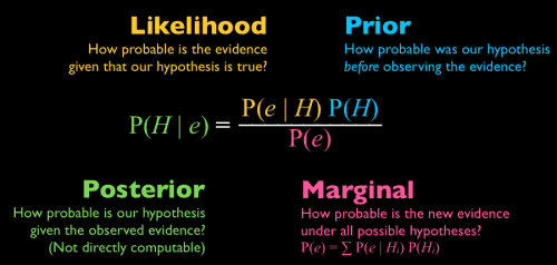
Bayesian statistics defines probability in terms of degree of belief. The more likely an outcome is the higher the degree of belief. In this context one of the most famous formulas of Bayesian statistics is the Bayes’ theorem. It links together four probabilities:
- Conditional probability of A given B – P (A|B)
- Probability of B given A – P (B|A)
- Unconditional probability of A – P (A)
- Unconditional probability of B – P (B)
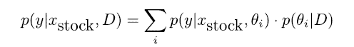
At the heart of fitting a Bayesian model is the Bayes’ theorem because it allows you to update predicted probabilities of an event by incorporating new information. For better understanding consider the following example. You are running a fund and need to forecast the future value of the S&P 500 Index, so you want p(y | xindex). You have several quants in your team. Each of your team members provides you with a different probabilistic prediction. Your best bet is to average out the predicted probabilities and give each p(y | xindex, θi) an appropriate weight. This weight should be proportional to the performance of each model on past data. This is the likelihood defined as p(D|θi). Additionally to that you add your judgement based on the models coming from your team members – prior p(θi). If you do not want to judge your experts you can instead give each of them the same subjective a priori judgement. This gives you the unnormalized posterior distribution. After normalizing it tells you to use the posterior as weights:
***
***
Explained in simple terms we use the wisdom of the crowd but weight the contributions of the individual experts. The quantity is called posterior because we determine it after we’ve seen the data.
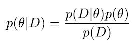
In order to determine P(θ |D) we need to determine the likelihood of the observed data P(D|θ), with parameter θ. We also need the prior P (θ) and evidence P(D). Since our training data D is fixed, P(D) is constant. If P(D) is constant it leads us to the fact that the posterior distribution is proportional to the likelihood times the prior: P(θ|D ) α P(D|θ) * P(θ).
Understanding Bayesian models with a coin toss example
Let’s start to fit our first Bayesian model with a coin toss example. There are two possible outcomes either y=1 (heads) or y=0 (tails). We want to determine the predictive distribution p(y) for the two outcomes. Normally we use input values for our model but in this case we have no input variables. We always toss the same coin. The only thing we need to estimate is an unconditional probability distribution for the outcome. For a fair coin the predictive distribution assigns a probability for 0.5 to heads and 0.5 to tails. On the other hand the epistemic uncertainty is zero.
Now let’s assume that we have a coin where we don’t know of whether it’s a fair coin or not. We are also unable to tell the exact value of θ. Therefore we need to estimate the probability for heads – θ = P(y = 1). We generate training data by throwing the coin three times and observe heads in all three instances. The first impression is that we have an unfair coin. But how sure can we be if we don’t have a lot of data? This is where we take the Bayesian approach.
We assume that we need to allow for some uncertainty about parameter θ. Instead of estimating an optimal value for the parameter we seek to determine the posterior distribution of the parameter. Our Bayes formula is:
***
***
- p(θ|D ) is the posterior
- p(D|θ) is the likelihood
- p(θ) is the prior
- p(D) is the marginal likelihood
We need to determine the joint likelihood p(D|θ) by multiplying all three observations:
***
P(D|θ) = P(y=1) * P(y=1) * P(y=1) = θ*θ*θ=θ3
***
We know that our parameter θ must be a number between 0 and 1 because it’s our probability for heads at each coin toss. If all values of θ are equally likely we have a uniform distribution. Since θ can take any value between 0 and 1, p(θ) is a continuous probability distribution.
We solve our coin toss example via brute force approximation. The following code shows you how to fit a Bernoulli distribution in the Bayesian way by using a brute force approach.
You can run the code in google colab.
Goal: Calculate the posterior distribution for the parameter θ as well as the predictive distribution for the outcome of a Bernoulli experiment. Use the brute force approach and pick different prior distributions for the parameter θ. We use discrete values for the prior and posterior of . We work with sums to approximate the integrals.
Try to understand the provided code by running it, checking the output and playing with it.
Dataset: You work with the observed values of coin tosses.
Steps:
- Define uniform prior for θ
- Evaluate joined likelihood and the unnormalized posterior at one specific θ
- Calculate joined likelihood, unnormalized posterior & normalized posterior for a range of θ
- Calculate and plot prior predictive distribution & posterior predictive distribution
try: #If running in colab
    import google.colab
    IN_COLAB = True
    %tensorflow_version 2.x
except:
    IN_COLAB = False
import tensorflow as tf
if (not tf.__version__.startswith('2')): #Checking if tf 2.0 is installed
    print('Please install tensorflow 2.0 to run this notebook')
print('Tensorflow version: ',tf.__version__, ' running in colab?: ', IN_COLAB)
if IN_COLAB:
    !pip install tensorflow_probability==0.8.0
import numpy as np

import tensorflow as tf
import tensorflow_probability as tfp

plt.style.use('default')
%matplotlib inline
tfd = tfp.distributions
print("TFP Version", tfp.__version__)
print("TF  Version",tf.__version__)
#Create train data. We set the outcome of three coin tosses to one, #meaning we get three times head
obs_data=np.repeat(1,3)
We first need to define a prior distribution for the parameter θ of the Bernoulli distribution. We evaluate the distributions at discrete points in the range 0.05 to 0.95. We use uniform prior where every theta has the same probability.
theta=np.arange(0.05,1,0.05)
print(theta)
prior = 1/len(theta) #The normalizing constant of the prior
#Evaluate joint likelihood and unnormalized posterior at one specific #$\theta = 0.5$
dist = tfp.distributions.Bernoulli(probs=0.5) #one specific theta
print(np.prod(dist.prob(obs_data))) #joint likelihood
print(np.prod(dist.prob(obs_data))*prior) #unnormalized posterior
#Repeat the process for all thetas, range 0.05 - 0.95
res = np.zeros((len(theta),5))
for i in range(0,len(theta)):
  dist = tfp.distributions.Bernoulli(probs=theta[i])
  res[i,0:4]=np.array((theta[i],np.prod(dist.prob(obs_data)),prior,np.prod(dist.prob(obs_data))*prior))
#Normalize posterior
import pandas as pd
res=pd.DataFrame(res,columns=["theta","jointlik","prior","unnorm_post","post"])
res["post"]=res["unnorm_post"]/np.sum(res["unnorm_post"])
res
#Plot prior and posterior for parameter θ
plt.figure(figsize=(16,6))
plt.subplot(1,2,1)
plt.stem(res["theta"],res["prior"])
plt.xlabel("theta")
plt.ylabel("probability")
plt.ylim([0,0.5])
plt.title("prior distribution")
plt.subplot(1,2,2)
plt.stem(res["theta"],res["post"])
plt.ylim([0,0.5])
plt.xlabel("theta")
plt.ylabel("probability")
plt.title("posterior distribution")
Posterior and prior for head
Predictive distribution:
For the probability of head, we have . For , we first use the posterior distribution resulting in
py1_post = np.sum((res["theta"])*res["post"])
py0_post = 1.0 - py1_post
py0_post, py1_post
py1_prior = np.sum((res["theta"])*res["prior"])
py0_prior = 1 - py1_prior
py0_prior, py1_prior
#Plot posterior and prior
plt.figure(figsize=(16,12))

plt.subplot(2,2,1)
plt.stem(res["theta"],res["prior"])
plt.xlabel("theta")
plt.ylabel("probability")
plt.ylim([0,0.5])
plt.title("prior distribution for theta")
plt.subplot(2,2,2)
plt.stem(res["theta"],res["post"])
plt.ylim([0,0.5])
plt.xlabel("theta")
plt.ylabel("probability")
plt.title("posterior distribution for theta")
plt.savefig("test.pdf")

plt.subplot(2,2,3)
plt.stem([0,1],[py0_prior,py1_prior])
plt.xlabel("Y")
plt.ylabel("P(y)")
plt.ylim([0,1])
plt.title("prior predictive distribution")
plt.subplot(2,2,4)
plt.stem([0,1],[py0_post,py1_post])
plt.ylim([0,1])
plt.xlabel("Y")
plt.ylabel("P(y)")
plt.title("posterior predictive distribution")


#plt.show()
plt.savefig("ch07_b2a.pdf")
# from google.colab import files
# files.download('ch07_b2a')
plt.show()
With this approach we sample the prior (θ) at 19 grid points (θ1=0.05, θ2=0.1,….θ19=). With the likelihoods of heads and posterior data we get:
p(y=1|D)=0.78
AND
p(y=0|D)=1-p(y=1|D)=0.22
Our predictive distribution based on the posterior tells us that we can expect heads with a 78% chances and tails with a probability of 22%.
***
Summary:
- Posterior gives more probability to parameter values that lead to higher likelihoods for the observed data.
- Bayes approach averages out all predicted distributions weighted with the posterior probabilities of the corresponding parameter values.
- Larger training data means smaller spread of the posterior.
- Larger training data smaller influence of prior.
- Posterior is a narrow Gaussian distribution for large training data sets.
- Brute force method can’t be used for complex problems like NN.
- Bayesian probabilistic models also capture epistemic uncertainty.
- Epistemic uncertainty is caused by uncertainty to the model parameter.
- Bayesian models replace each parameter by a distribution.
- Bayesian model shows a better prediction compared to non-Bayesian models when training data is limited.
***
————-
Reference
Oliver Dürr, Beate Sick and Elvis Murina. (2020). Probabilistic Deep Learning. Manning Publications.
Eugene Charniak(2019). Introduction to Deep Learning. The MIT Press.