

Identifying Anomalies in Capital Markets: Accrual Anomaly
Since the financial crisis in 2008 the number of anomaly related academic papers exploded and has grown so quickly that it is impossible to keep up with the full scope of research. To accommodate the need of an overview in this interesting research field we will summarize the most prominent market anomalies and present our findings in a series of articles. We start our series with the accrual anomaly which has been the subject of many academic research papers.
If we look close enough we can find unexpected price behavior in financial markets that can be exploited by the savvy investor to earn abnormal returns. Every anomaly is a deviation from the efficient market theory. The efficient market hypothesis is a hypothesis that states that share prices reflect all information and consistent alpha generation is impossible. While academics point to a large body of evidence in support of this theory, an equal amount of disagreement also exists. Investors like Peter Lynch, David Tepper and Ed Thorp have consistently beaten the market by long periods, which by definition is impossible according to the efficient market theory. There are no free lunches on Wall Street but tradeable anomalies seem to persist in the markets. A caveat at this point, anomalies can appear, disappear or reappear. It is important to have a system in place that identifies these patterns and evaluates the validity of market anomalies on a continuous basis.
When searching for anomalies the first step in the process is identifying a mispricing signal. The second step consists of evaluating the statistical reliability of a mispricing signal. When trading stocks the typical approach is sorting the cross section of companies into, for example, deciles based on a mispricing signal. The statistical reliability can be measured by analyzing the alpha the strategy generates over the tested time frame. If the variation of risk adjusted returns is low across the backtested time frame the strategy would be considered statistically reliable. A t-statistic with a p-value of less than 5% can be used as a statistically reliable criterion of an alpha.
Among all the market anomalies and market inefficiencies the most unique among them is the accrual anomaly. When it was discovered it was the most robust anomaly for a long period of time. Unfortunately, this price behavior has gradually declined since its discovery but remember anomalies can appear, disappear and reappear. Despite the fact that it is not effective as it used to be doesn’t mean you shouldn’t keep an eye on this market phenomenon or maybe tweak a few parameters to improve its predictability.
What are accruals?
The accounting term accruals refers to adjustments that must be made before a company’s financial statements are issued. Accruals involve following business transactions:
- expenses, losses, and liabilities that have been incurred but are not yet recorded in the accounts, and
- revenues and assets that have been earned but are not yet recorded in the accounts.
Example
In order to illustrate exactly what accruals are and how they affect earnings, we begin with a simple example. Let us assume that Peter and Paul are two budding entrepreneurs who each decide to set up lemonade stands. Peter starts his first day of business by buying $100 of lemonade, $10 of cups and renting a lemonade stand for $10/day. This costs him a total of $120, all of which he pays for in cash. By the end of the day, he has sold all of his lemonade and used all his cups. All of his customers pay him in cash and his total cash proceeds are $200. The exhibit below summarizes the financial statements that Peter produces at the end of this first day. (Sloan et al., 1996, p. 2)
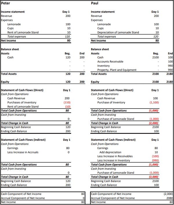
His first day’s earnings are pretty simple to compute. He ends the day with net income of $200-$120=$80. Peter’s balance sheet is also very simple. Peter started his business by contributing $120 in cash (the other side of the balance sheet records his equity ownership stake). He finished the first day with $200 in cash, and so his earnings were $80, his operating cash flows were $80 and his equity ownership stake increased by $80. Paul, on the other hand, starts his first day by buying $1,000 of lemonade, $100 of cups and a fancy new lemonade stand for $1,000. This costs him a total of $2,100, all of which he pays for in cash. By the end of the first day, he has sold about 10% of his lemonade and has used up about 10% of his cups. Paul also sold his lemonade for a total of $200, but half of his customers were short on cash and so he agreed that they could stop by and pay him the next day, collecting only $100 in cash on his first day. His lemonade stand is now a bit sticky, but it is holding up well and he hopes to get a further 99 days of usage out of it. Unlike Peter, Paul needs an accountant to help him determine his earnings. One thing he knows for sure is that he is now out of pocket $2,000 in cash, since he had to invest $2,100 to start the business and only collected $100 of cash on the first day. But he still has heaps of lemonade and cups and a nearly-new lemonade stand. Paul’s accountant tells him that since he sold about 10% of his lemonade and used about 10% of his cups, the remaining lemonade is worth about $900 and the remaining cups are worth about $90, so Paul has $990 worth of ‘inventory’. Paul explains to his accountant that he is still owed $100 for the day’s lemonade sales and that he expects to collect the cash tomorrow. The accountant says ‘are you sure these customers will come back and pay you?’ Paul says ‘are you calling me a liar?’ at which point the accountant promptly tells Paul that he also has $100 worth of ‘accounts receivable’. The accountant also notices the sticky lemonade stand and says ‘is this yours?’ Paul says ‘yes, and I expect to get another 99 days use out of that beauty’, upon which the accountant tells Paul that he has ‘property, plant & equipment’ worth $990. After hitting a few buttons on his calculator, the accountant tells Paul he now has a balance sheet with $2,080 worth of non-cash assets ($990 of inventory plus $100 of 3 accounts receivable plus $990 of fixed assets). When Paul started the day, he had no noncash assets. The increase in non-cash assets for the period is therefore $2,080. This increase in non-cash assets represents the accruals for the period. The accountant tells Paul that a quick way to figure out his earnings for the period is to add the accruals to the net cash flows for the period. Cash is -$2,000 and accruals are $2,080, and so his first day’s net income is also $80. (Sloan et al., 1996, p. 3)
To summarize the research findings we can argue that if a stock has high earnings today, we can expect that it will stay high in the future. To assess the probability of earnings staying high, we can check if current earnings are driven by accruals of cash flows. If the earnings are driven by accruals it is less likely that earnings will stay high. Generally speaking high earnings paired with high accruals are a warning sign.
An updated version of Sloan’s test uses the following parameters:
- Compute accruals for a sample of stocks between 1970 and 2007.
- Rank observations from lowest to highest based on accruals.
- Firm years are assigned into deciles based on the rank of accruals. Decile 1 consists of lowest ranked 10% and decile 10 of the highest ranked 10%.
- Calculate annual stock returns beginning 4 months after the fiscal year ends.
- Calculate equally weighted portfolio returns for each accrual decile.
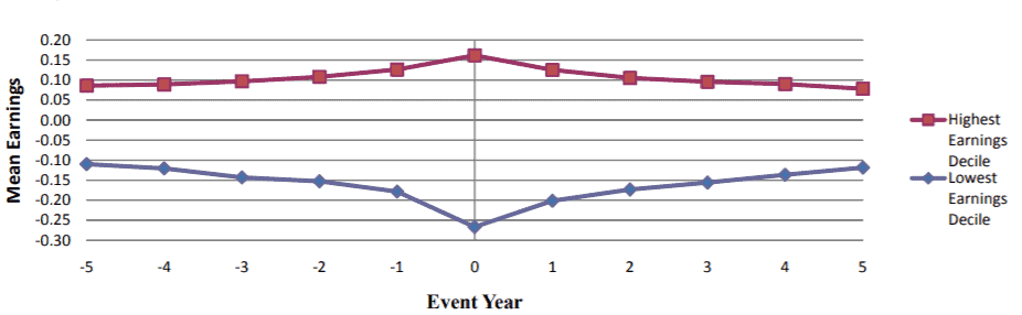
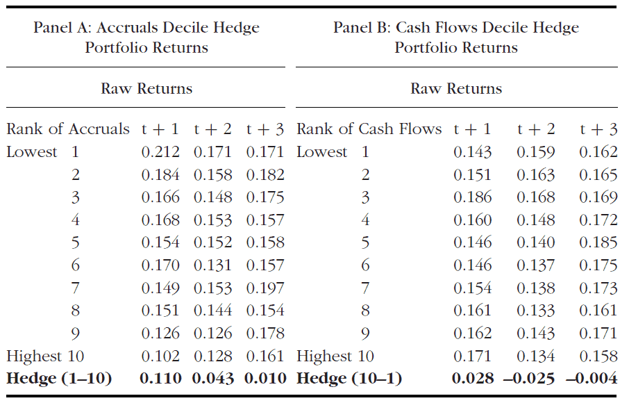
The results show that the highest accrual portfolio has the lowest future return in year t+1 and t+2. The strength of these returns is weaker then it was originally reported by Sloan. The lowest bottom – see table below – shows hedge returns to an investment strategy of going long in the lowest accrual portfolio and short in the highest accrual portfolio. The return is 11% over the subsequent year (Zacks, 2011, p.35).
Since the publication of this research the accrual anomaly has been arbitraged away by institutional investors. However, it doesn’t mean that the accrual anomaly can’t be exploited with a few parameter adjustments as we show next.
Summary of key findings:
- It is important to differentiate between the main drivers of extreme accruals before jumping to conclusions about the quality of earnings. Change in accounting procedure vs. Result of slowing demand/inventory buildups – these are completely different reasons of extreme accruals.
- Sell-side analysts fixate on earnings. Findings by Bradshaw et al. found that analysts’ earnings forecasts for companies with high accruals were initially too optimistic.
- Inventory accruals exhibit the most robust relation with future stock returns.
- Higher accrual companies are more likely to have subsequent SEC enforcement actions.
- Stronger accrual anomaly among profit-firms, large-sized firms and firms with higher covariation between accruals and the employment growth rate, and firms with higher earnings response coefficients (Ran et al. , 2020).
Can you make money from the accrual anomaly? Let’s find out. For the backtest we calculate accrual anomalies using balance sheet data.
Calculating accruals:
Balance sheet based accruals (the non-cash component of earnings) are calculated as:
BS_ACC = ( ∆CA – ∆Cash) – ( ∆CL – ∆STD – ∆ITP) – Dep
∆CA = annual change in current assets
∆Cash = change in cash and cash equivalents
∆CL = change in current liabilities
∆STD = change in debt included in current liabilities
∆ITP = change in income taxes payable
Dep = annual depreciation and amortization expense
Stocks are then sorted into deciles. Long stocks with the lowest accruals and short stocks with the highest accruals. The portfolio is rebalanced yearly in June (after all companies publish their earnings).
def CoarseSelectionFunction(self, coarse):
        if self.yearly_rebalance:
            self.filtered_coarse = [x.Symbol for x in coarse if (x.HasFundamentalData)
                                                            and (x.Market == "usa")]
            return self.filtered_coarse
        else:
            return []

def FineSelectionFunction(self, fine):
    if self.yearly_rebalance:
        fine = [x for x in fine if (float(x.FinancialStatements.BalanceSheet.CurrentAssets.Value) > 0)
                                and (float(x.FinancialStatements.BalanceSheet.CashAndCashEquivalents.Value) > 0)
                               and (float(x.FinancialStatements.BalanceSheet.CurrentLiabilities.Value) > 0)
                                and (float(x.FinancialStatements.BalanceSheet.CurrentDebt.Value) > 0)
                                and (float(x.FinancialStatements.BalanceSheet.IncomeTaxPayable.Value) > 0)
                                and (float(x.FinancialStatements.IncomeStatement.DepreciationAndAmortization.Value) > 0)]

        if not self.previous_fine:
            self.previous_fine = fine
            self.yearly_rebalance = False
            return []
        else:
            self.filtered_fine = self.CalculateAccruals(fine,self.previous_fine)
            sorted_filter = sorted(self.filtered_fine, key=lambda x: x.bs_acc)
            self.filtered_fine = [i.Symbol for i in sorted_filter]
            self.previous_fine = fine
            return self.filtered_fine
    else:
        return []
Stocks from the previous and current year are selected and their balance sheet based accrual values are calculated. We sort the stocks in ascending order based upon the implemented formula. We account for size difference across the sample firms by scaling the accruals by the average of the beginning and end-of-year book value of total assets.
def CalculateAccruals(self, current, previous):
    accruals = []
    for stock_data in current:
        try:
            prev_data = None
            for x in previous:
                if x.Symbol == stock_data.Symbol:
                    prev_data = x
                    break

            delta_assets = float(stock_data.FinancialStatements.BalanceSheet.CurrentAssets.Value)-float(prev_data.FinancialStatements.BalanceSheet.CurrentAssets.Value)
            delta_cash = float(stock_data.FinancialStatements.BalanceSheet.CashAndCashEquivalents.Value)-float(prev_data.FinancialStatements.BalanceSheet.CashAndCashEquivalents.Value)
            delta_liabilities = float(stock_data.FinancialStatements.BalanceSheet.CurrentLiabilities.Value)-float(prev_data.FinancialStatements.BalanceSheet.CurrentLiabilities.Value)
            delta_debt = float(stock_data.FinancialStatements.BalanceSheet.CurrentDebt.Value)-float(prev_data.FinancialStatements.BalanceSheet.CurrentDebt.Value)
            delta_tax = float(stock_data.FinancialStatements.BalanceSheet.IncomeTaxPayable.Value)-float(prev_data.FinancialStatements.BalanceSheet.IncomeTaxPayable.Value)
            dep = float(stock_data.FinancialStatements.IncomeStatement.DepreciationAndAmortization.Value)
            avg_total = (float(stock_data.FinancialStatements.BalanceSheet.TotalAssets.Value)+float(prev_data.FinancialStatements.BalanceSheet.TotalAssets.Value))/2

            stock_data.bs_acc = ((delta_assets-delta_cash)-(delta_liabilities-delta_debt-delta_tax)-dep)/avg_total
            accruals.append(stock_data)
        except:
            pass
    return accruals
The portfolio is balanced every year in June. With the function OnData() the top decile of stocks is shorted and the bottom decile of stocks is entered long.
Complete code (can be executed via quantconnect)
class NetCurrentAssetValue(QCAlgorithm):

    def Initialize(self):
        #rebalancing should occur in July
        self.SetStartDate(2007,5,15)  #Set Start Date
        self.SetEndDate(2018,7,15)    #Set End Date
        self.SetCash(1000000)           #Set Strategy Cash
        self.UniverseSettings.Resolution = Resolution.Daily
        self.previous_fine = None
        self.filtered_fine = None
        self.AddUniverse(self.CoarseSelectionFunction,self.FineSelectionFunction)
        self.AddEquity("SPY", Resolution.Daily)
        #monthly scheduled event but will only rebalance once a year
        self.Schedule.On(self.DateRules.MonthStart("SPY"), self.TimeRules.At(23, 0), self.rebalance)
        self.months = -1
        self.yearly_rebalance = False

    def CoarseSelectionFunction(self, coarse):
        if self.yearly_rebalance:
            # drop stocks which have no fundamental data
            self.filtered_coarse = [x.Symbol for x in coarse if (x.HasFundamentalData)
                                                            and (x.Market == "usa")]
            return self.filtered_coarse
        else:
            return []

    def FineSelectionFunction(self, fine):
        if self.yearly_rebalance:
            #filters out the companies that don't contain the necessary data
            fine = [x for x in fine if (float(x.FinancialStatements.BalanceSheet.CurrentAssets.Value) > 0)
                                    and (float(x.FinancialStatements.BalanceSheet.CashAndCashEquivalents.Value) > 0)
                                   and (float(x.FinancialStatements.BalanceSheet.CurrentLiabilities.Value) > 0)
                                    and (float(x.FinancialStatements.BalanceSheet.CurrentDebt.Value) > 0)
                                    and (float(x.FinancialStatements.BalanceSheet.IncomeTaxPayable.Value) > 0)
                                    and (float(x.FinancialStatements.IncomeStatement.DepreciationAndAmortization.Value) > 0)]

            if not self.previous_fine:
                #will wait one year in order to have the historical fundamental data
                self.previous_fine = fine
                self.yearly_rebalance = False
                return []
            else:
                #will calculate and sort the balance sheet accruals
                self.filtered_fine = self.CalculateAccruals(fine,self.previous_fine)
                sorted_filter = sorted(self.filtered_fine, key=lambda x: x.bs_acc)
                self.filtered_fine = [i.Symbol for i in sorted_filter]
                #we save the fine data for the next year's analysis
                self.previous_fine = fine
                return self.filtered_fine
        else:
            return []

    def CalculateAccruals(self, current, previous):
        accruals = []
        for stock_data in current:
            #compares this and last year's fine fundamental objects
            try:
                prev_data = None
                for x in previous:
                    if x.Symbol == stock_data.Symbol:
                        prev_data = x
                        break

                #calculates the balance sheet accruals and adds the property to the fine fundamental object
                delta_assets = float(stock_data.FinancialStatements.BalanceSheet.CurrentAssets.Value)-float(prev_data.FinancialStatements.BalanceSheet.CurrentAssets.Value)
                delta_cash = float(stock_data.FinancialStatements.BalanceSheet.CashAndCashEquivalents.Value)-float(prev_data.FinancialStatements.BalanceSheet.CashAndCashEquivalents.Value)
                delta_liabilities = float(stock_data.FinancialStatements.BalanceSheet.CurrentLiabilities.Value)-float(prev_data.FinancialStatements.BalanceSheet.CurrentLiabilities.Value)
                delta_debt = float(stock_data.FinancialStatements.BalanceSheet.CurrentDebt.Value)-float(prev_data.FinancialStatements.BalanceSheet.CurrentDebt.Value)
                delta_tax = float(stock_data.FinancialStatements.BalanceSheet.IncomeTaxPayable.Value)-float(prev_data.FinancialStatements.BalanceSheet.IncomeTaxPayable.Value)
                dep = float(stock_data.FinancialStatements.IncomeStatement.DepreciationAndAmortization.Value)
                avg_total = (float(stock_data.FinancialStatements.BalanceSheet.TotalAssets.Value)+float(prev_data.FinancialStatements.BalanceSheet.TotalAssets.Value))/2
                #accounts for the size difference
                stock_data.bs_acc = ((delta_assets-delta_cash)-(delta_liabilities-delta_debt-delta_tax)-dep)/avg_total
                accruals.append(stock_data)
            except:
                #value in current universe does not exist in the previous universe
                pass
        return accruals

    def rebalance(self):
        #yearly rebalance
        self.months+=1
        if self.months%12 == 0:
            self.yearly_rebalance = True

    def OnData(self, data):
        if not self.yearly_rebalance: return
        if self.filtered_fine:
            portfolio_size = int(len(self.filtered_fine)/10)
            #pick the upper decile to short and the lower decile to long
            short_stocks = self.filtered_fine[-portfolio_size:]
            long_stocks = self.filtered_fine[:portfolio_size]
            stocks_invested = [x.Key for x in self.Portfolio]
            for i in stocks_invested:
                #liquidate the stocks not in the filtered balance sheet accrual list
                if i not in self.filtered_fine:
                    self.Liquidate(i)
                #long the stocks in the list
                elif i in long_stocks:
                    self.SetHoldings(i, 1/(portfolio_size*2))
                #short the stocks in the list
                elif i in short_stocks:
                    self.SetHoldings(i,-1/(portfolio_size*2))
            self.yearly_rebalance = False
            self.filtered_fine = False
Strategy results
| PSR | 0 | Sharpe Ratio | 0.407 |
| Total Trades | 1060 | Average Win | 0.75% |
| Average Loss | -0.83% | Compounding Annual Return | 5.980% |
| Drawdown | 39.100% | Expectancy | -0.130 |
| Net Profit | 120.814% | PSR | 0.697% |
| Loss Rate | 54% | Win Rate | 46% |
| Profit-Loss Ratio | 0.90 | Alpha | 0.062 |
| Beta | -0.019 | Annual Standard Deviation | 0.149 |
| Annual Variance | 0.022 | Information Ratio | -0.132 |
| Tracking Error | 0.241 | Treynor Ratio | -3.162 |
| Total Fees | $6479.89 |
Equity graph

Conclusion
Based on our tests we show that tweaking a few paramters makes this strategy profitable again. Another way of exploiting this anomaly is by trading options on stocks showing up on the list of accrual anomalies by buying puts for the top decile of stocks and buying calls for the bottom decile of stocks. This strategy should yield some robust results as well.
– – – –
References
AN, Ran and Chiu, Peng-Chia and Zhang, Yinglei. (2020). Back to Fundamentals: The Accrual–Cash Flow Correlation, the Inverted-U Pattern, and Stock Returns.
Bradshaw, M. T., S. A. Richardson, and R. G. Sloan. (2001). Do analysts and
auditors use information in accruals? Journal of Accounting Research
39 (1): 45–74.
Sloan, R. G. (1996). Do stock prices fully reflect information in accruals
and cash flows about future earnings? The Accounting Review 71 (3):
289–315.
Zacks, L. (2011). The handbook of equity market anomalies: translating market inefficiencies into effective investment strategies.