

The Complete Guide to Portfolio Optimization in R PART2
Congratulations you made it to part2 of our tutorial. Give yourself a round of applause. If you stumbled upon part2 before reading part1 we advise you to start from the beginning and read part1 first.
In Part2 we dive into mean variance portfolio optimization, mean CVar portfolios and backtesting. As mentioned in part1 we conclude this tutorial with a full blown portfolio optimization process with a real world example. After going through all of the content you should have acquired profound knowledge of portfolio optimization in R and be able to optimize any kind of portfolio with your eyes closed.
Content
PART1:
- Working with data
- Loading times series data sets
- Reading data from CSV files
- Downloading data from the internet
- Modifying time series data
- Sample time series data randomly
- Sorting in ascending order
- Reverse data
- Alignment of timeSeries objects
- Merging time series data
- Binding time series
- Merging columns and rows
- Subsetting data and replacing parts of a data set
- Find first and last records in a time series
- Subset by column names
- Extract specific date
- Aggregating data
- Computing rolling statistics
- Manipulate data with financial functions
- Robust statistical methods
- Implementing the portfolio framework
PART2:
- Representing data with timeSeries objects
- Set portfolio constraints
- Optimizing a portfolio
- Case study portfolio optimization
- Portfolio backtesting
- What to do next
Representing data with timeSeries objects
With S4 timeSeries objects found in the rmetrics package we can represent data for portfolio optimization. To create an S4 object of class fPFOLIODATA we use the function portfolioData().
>showClass("fPFOLIODATA")
Class "fPFOLIODATA" [package "fPortfolio"]

Slots:

Name:        data statistics   tailRisk
Class:       list       list       list
The function portfolioData() allows us to define data settings that we can use in portfolio functions. To illustrate this with an example we use the LPP2005.RET data set working with columns “SBI”,”SPI”,”LMI” and “MPI”. We create a portfolio object with the data set and the default portfolio specification.
>args(portfolioData)
function (data, spec = portfolioSpec())
NULL
>lppAssets <- 100 * LPP2005.RET[, c("SBI", "SPI", "LMI", "MPI")]
>lppData <- portfolioData(data = lppAssets, spec = portfolioSpec())
With the function str() we take a look inside the data structure of a portfolio.
>str(lppData, width = 65, strict.width = "cut")
Formal class 'fPFOLIODATA' [package "fPortfolio"] with 3 slots
  ..@ data      :List of 3
  .. ..$ series :Time Series:
 Name:               object
Data Matrix:
 Dimension:          377 4
 Column Names:       SBI SPI LMI MPI
 Row Names:          2005-11-01  ...  2007-04-11
Positions:
 Start:              2005-11-01
 End:                2007-04-11
With:
 Format:             %Y-%m-%d
 FinCenter:          GMT
 Units:              SBI SPI LMI MPI
 Title:              Time Series Object
 Documentation:      Tue Jan 20 17:49:06 2009 by user:
  .. ..$ nAssets: int 4
  .. ..$ names  : chr [1:4] "SBI" "SPI" "LMI" "MPI"
  ..@ statistics:List of 5
  .. ..$ mean     : Named num [1:4] 4.07e-05 8.42e-02 5.53e-03 ..
  .. .. ..- attr(*, "names")= chr [1:4] "SBI" "SPI" "LMI" "MPI"
  .. ..$ Cov      : num [1:4, 1:4] 0.0159 -0.0127 0.0098 -0.015..
  .. .. ..- attr(*, "dimnames")=List of 2
  .. .. .. ..$ : chr [1:4] "SBI" "SPI" "LMI" "MPI"
  .. .. .. ..$ : chr [1:4] "SBI" "SPI" "LMI" "MPI"
  .. ..$ estimator: chr "covEstimator"
  .. ..$ mu       : Named num [1:4] 4.07e-05 8.42e-02 5.53e-03 ..
  .. .. ..- attr(*, "names")= chr [1:4] "SBI" "SPI" "LMI" "MPI"
  .. ..$ Sigma    : num [1:4, 1:4] 0.0159 -0.0127 0.0098 -0.015..
  .. .. ..- attr(*, "dimnames")=List of 2
  .. .. .. ..$ : chr [1:4] "SBI" "SPI" "LMI" "MPI"
  .. .. .. ..$ : chr [1:4] "SBI" "SPI" "LMI" "MPI"
  ..@ tailRisk  : list()
With the command print(lppData) we can print a portfolio data object. The output prints the first and last three lines of the data set alongside the sample mean and covariance estimates found in the @statistics slot.
>print(lppData)

Head/Tail Series Data:

GMT
                  SBI       SPI        LMI       MPI
2005-11-01 -0.0612745 0.8414595 -0.1108882 0.1548062
2005-11-02 -0.2762009 0.2519342 -0.1175939 0.0342876
2005-11-03 -0.1153092 1.2707292 -0.0992456 1.0502959
GMT
                  SBI        SPI        LMI        MPI
2007-04-09  0.0000000  0.0000000 -0.1032441  0.8179152
2007-04-10 -0.0688995  0.6329425 -0.0031500 -0.1428291
2007-04-11  0.0306279 -0.1044170 -0.0090900 -0.0991064

Statistics:

$mean
         SBI          SPI          LMI          MPI
0.0000406634 0.0841754390 0.0055315332 0.0590515119

$Cov
             SBI         SPI          LMI         MPI
SBI  0.015899554 -0.01274142  0.009803865 -0.01588837
SPI -0.012741418  0.58461212 -0.014074691  0.41159843
LMI  0.009803865 -0.01407469  0.014951108 -0.02332223
MPI -0.015888368  0.41159843 -0.023322233  0.53503263

$estimator
[1] "covEstimator"

$mu
         SBI          SPI          LMI          MPI
0.0000406634 0.0841754390 0.0055315332 0.0590515119

$Sigma
             SBI         SPI          LMI         MPI
SBI  0.015899554 -0.01274142  0.009803865 -0.01588837
SPI -0.012741418  0.58461212 -0.014074691  0.41159843
LMI  0.009803865 -0.01407469  0.014951108 -0.02332223
MPI -0.015888368  0.41159843 -0.023322233  0.53503263
The S4 time series object is kept in the @data slot. We can extract the content with the function getData().
>Data <- portfolioData(lppData)
>getData(Data)[-1]
$nAssets
[1] 4

$names
[1] "SBI" "SPI" "LMI" "MPI"
The content of the @statistics slot holds information on the mean and covariance matrix and can be called with the getStatistics() function.
>getStatistics(Data)
$mean
         SBI          SPI          LMI          MPI
0.0000406634 0.0841754390 0.0055315332 0.0590515119

$Cov
             SBI         SPI          LMI         MPI
SBI  0.015899554 -0.01274142  0.009803865 -0.01588837
SPI -0.012741418  0.58461212 -0.014074691  0.41159843
LMI  0.009803865 -0.01407469  0.014951108 -0.02332223
MPI -0.015888368  0.41159843 -0.023322233  0.53503263

$estimator
[1] "covEstimator"

$mu
         SBI          SPI          LMI          MPI
0.0000406634 0.0841754390 0.0055315332 0.0590515119

$Sigma
             SBI         SPI          LMI         MPI
SBI  0.015899554 -0.01274142  0.009803865 -0.01588837
SPI -0.012741418  0.58461212 -0.014074691  0.41159843
LMI  0.009803865 -0.01407469  0.014951108 -0.02332223
MPI -0.015888368  0.41159843 -0.023322233  0.53503263
Set portfolio constraints
By using constraints we are defining restrictions on portfolio weights. In the rmetrics package the function portfolioConstraints() creates the default settings and reports on all constraints.
>showClass("fPFOLIOCON")
Class "fPFOLIOCON" [package "fPortfolio"]

Slots:

Name:    stringConstraints     minWConstraints     maxWConstraints   eqsumWConstraints
Class:           character             numeric             numeric              matrix

Name:   minsumWConstraints  maxsumWConstraints     minBConstraints     maxBConstraints
Class:              matrix              matrix             numeric             numeric

Name:     listFConstraints     minFConstraints     maxFConstraints minBuyinConstraints
Class:                list             numeric             numeric             numeric

Name:  maxBuyinConstraints    nCardConstraints  minCardConstraints  maxCardConstraints
Class:             numeric             integer             numeric             numeric
The function portfolioConstraints() consists of the following arguments:
Argument: constraints
Values:
- “LongOnly” long-only constraints [0,1]
- “Short” unlimited short selling, [-Inf,Inf]
- “minW[<…>]=<…> lower box bounds
- “maxw[<…>]=<…> upper box bounds
- “minsumW[<…>]=<…> lower group bounds
- “maxsumW[<…>]=<…> upper group bounds
- “minB[<…>]=<…> lower covariance risk budget bounds
- “maxB[<…>]=<…> upper covariance risk budget bounds
- “listF=list(<…>)” list of non-linear functions
- “minf[<…>]=<…>” lower non-linear function bounds
- “maxf[<…>]=<…>” upper covariance risk budget
Constructing portfolio constraints
The example below creates Long-only settings for returns from the LPP2005 data set ,displays the structure of a portfolio constrains object and prints the results.
>Data <- 100 * LPP2005.RET[, 1:3]
>Spec <- portfolioSpec()
>setTargetReturn(Spec) <- mean(Data)
>Constraints <- "LongOnly"
>defaultConstraints <- portfolioConstraints(Data, Spec, Constraints)
>str(defaultConstraints, width = 65, strict.width = "cut")
Formal class 'fPFOLIOCON' [package "fPortfolio"] with 16 slots
  ..@ stringConstraints  : chr "LongOnly"
  ..@ minWConstraints    : Named num [1:3] 0 0 0
  .. ..- attr(*, "names")= chr [1:3] "SBI" "SPI" "SII"
  ..@ maxWConstraints    : Named num [1:3] 1 1 1
  .. ..- attr(*, "names")= chr [1:3] "SBI" "SPI" "SII"
  ..@ eqsumWConstraints  : num [1:2, 1:4] 3.60e-02 -1.00 4.07e-..
  .. ..- attr(*, "dimnames")=List of 2
  .. .. ..$ : chr [1:2] "Return" "Budget"
  .. .. ..$ : chr [1:4] "ceq" "SBI" "SPI" "SII"
  ..@ minsumWConstraints : logi [1, 1] NA
  ..@ maxsumWConstraints : logi [1, 1] NA
  ..@ minBConstraints    : Named num [1:3] -Inf -Inf -Inf
  .. ..- attr(*, "names")= chr [1:3] "SBI" "SPI" "SII"
  ..@ maxBConstraints    : Named num [1:3] 1 1 1
  .. ..- attr(*, "names")= chr [1:3] "SBI" "SPI" "SII"
  ..@ listFConstraints   : list()
  ..@ minFConstraints    : num(0)
  ..@ maxFConstraints    : num(0)
  ..@ minBuyinConstraints: Named num [1:3] 0 0 0
  .. ..- attr(*, "names")= chr [1:3] "SBI" "SPI" "SII"
  ..@ maxBuyinConstraints: Named num [1:3] 1 1 1
  .. ..- attr(*, "names")= chr [1:3] "SBI" "SPI" "SII"
  ..@ nCardConstraints   : int 3
  ..@ minCardConstraints : Named num [1:3] 0 0 0
  .. ..- attr(*, "names")= chr [1:3] "SBI" "SPI" "SII"
  ..@ maxCardConstraints : Named num [1:3] 1 1 1
  .. ..- attr(*, "names")= chr [1:3] "SBI" "SPI" "SII"
>print(defaultConstraints)

Title:
 Portfolio Constraints

Lower/Upper Bounds:
      SBI SPI SII
Lower   0   0   0
Upper   1   1   1

Equal Matrix Constraints:
               ceq          SBI         SPI         SII
Return  0.03603655  4.06634e-05  0.08417544  0.02389356
Budget -1.00000000 -1.00000e+00 -1.00000000 -1.00000000

Cardinality Constraints:
      SBI SPI SII
Lower   0   0   0
Upper   1   1   1
To consider another example we can use short selling constraints instead of a long-only portfolio.
>shortConstraints <- "Short"
>portfolioConstraints(Data, Spec, shortConstraints)

Title:
 Portfolio Constraints

Lower/Upper Bounds:
       SBI  SPI  SII
Lower -Inf -Inf -Inf
Upper  Inf  Inf  Inf

Equal Matrix Constraints:
               ceq          SBI         SPI         SII
Return  0.03603655  4.06634e-05  0.08417544  0.02389356
Budget -1.00000000 -1.00000e+00 -1.00000000 -1.00000000

Cardinality Constraints:
      SBI SPI SII
Lower   0   0   0
Upper   1   1   1
Using box constraints and setting the lower bounds to negative values we can implement arbitrary short selling. With the two character strings minW and maxW we can limit the portfolio weights by lower and upper bounds.
>box.1 <- "minW[1:3] = 0.1"
>box.2 <- "maxW[c(1,3)] = c(0.5, 0.6)"
>box.3 <- "maxW[2] = 0.4"
>boxConstraints <- c(box.1, box.2, box.3)
>boxConstraints
[1] "minW[1:3] = 0.1"            "maxW[c(1,3)] = c(0.5, 0.6)" "maxW[2] = 0.4"
> portfolioConstraints(Data, Spec, boxConstraints)

Title:
 Portfolio Constraints

Lower/Upper Bounds:
      SBI SPI SII
Lower 0.1 0.1 0.1
Upper 0.5 0.4 0.6

Equal Matrix Constraints:
               ceq          SBI         SPI         SII
Return  0.03603655  4.06634e-05  0.08417544  0.02389356
Budget -1.00000000 -1.00000e+00 -1.00000000 -1.00000000

Cardinality Constraints:
      SBI SPI SII
Lower   0   0   0
Upper   1   1   1
The constraints above tell us that we want to invest a minimum of 10% in each asset (see lower bound 0.1, 0.1, 0.1) and not more than 50% in the first asset. A 40% maximum investment for the second asset and 60% maximum investment in the third asset. Another method that we can use is to define the total weight of a group of assets. We can use the following strings to set group constraints:
Constraints Settings:
- “eqsumW” equality group constraints #total amount invested in a group of assets
- “minsumW” lower bounds group constraints
- “maxsumw” upper bounds group constraints
>group.1 <- "eqsumW[c(1,3)]=0.6"
>group.2 <- "minsumW[c(2,3)]=0.2"
>group.3 <- "maxsumW[c(1,2)]=0.7"
>groupConstraints <- c(group.1, group.2, group.3)
>groupConstraints
[1] "eqsumW[c(1,3)]=0.6"  "minsumW[c(2,3)]=0.2" "maxsumW[c(1,2)]=0.7"
>portfolioConstraints(Data, Spec, groupConstraints)

Title:
 Portfolio Constraints

Lower/Upper Bounds:
      SBI SPI SII
Lower   0   0   0
Upper   1   1   1

Equal Matrix Constraints:
               ceq          SBI         SPI         SII
Return  0.03603655  4.06634e-05  0.08417544  0.02389356
Budget -1.00000000 -1.00000e+00 -1.00000000 -1.00000000
eqsumW  0.60000000  1.00000e+00  0.00000000  1.00000000

Lower Matrix Constraints:
      avec SBI SPI SII
lower  0.2   0   1   1

Upper Matrix Constraints:
      avec SBI SPI SII
upper  0.7   1   1   0

Cardinality Constraints:
      SBI SPI SII
Lower   0   0   0
Upper   1   1   1
The first string means that we invest 60% in asset 1 and 3. For group.2 we invest a minimum of 20% in asset 2 and 3. For group.3 we invest a maximum of 70% in asset 1 and 2.
Set lower and upper bounds
Probably the question running through your mind is, “Sounds interesting but how can I know how to set lower and upper bounds?” This is up to you to decide. However, more often than not the simplest solutions work best. For example, if you are about to set the weights for a sector the best way forward would be to construct spread indices of the sectors you want to invest your money in. Mr. Market already showed us numerous times that when volatility in the market crests, the performance of all stocks tends to be highly correlated. Stocks in different sectors start to wander when volatility goes down and things magically become less correlated. The graph below illustrates this phenomenon. Take a close look.
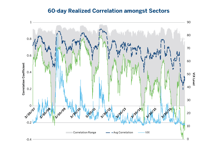
The blue dotted line shows the average correlation for all pairs of sectors based on the S&P Select Sector Indexes. The shaded area shows the correlation amongst different sectors. As we can see sectors tend to decouple when volatility subsides. In order to measure if a sector is “overbought” or “oversold” we can construct a spread between two sectors. Of course there is not a “best way” to construct these sector spreads so they should only be used as a guideline for defining meaningful portfolio weights. By way of example, if a portfolio manager has a view that the technology sector will underperform the market while the energy sector will outperform the market, one can conceivably buy $1 million of the energy sector exposure while short selling $1 million of the technology sector. By using the following equation we can find more relevant coefficients:

We estimate β by regressing the historical returns of the sector on those of the overall market. We can set the exposure in Sector A to one dollar and µ dollar of exposure is sold in Sector B. The total sensitivity to the market returns is defined as (βA–μβB). We eliminate exposure to the overall market by setting µ:
In this example µ is greater than 1 if B is less sensitive than sector A to the overall market return. Translated into trader language it means that we have to adjust our B sector position upward. This is your guideline. The fine tuning happens during the portfolio optimization process. If you want to elaborate on this further we advise you to read the article on the CME website.
Optimizing a portfolio
With the following portfolio optimization functions we compute or optimize a single portfolio. These functions are part of the fPortfolio package.
Portfolio Functions:
- feasiblePortfolio: returns a feasible portfolio given the
- vector of portfolio weights
- efficientPortfolio: returns the portfolio with the lowest risk for a given target return
- maxratioPortfolio: returns the portfolio with the highest return/risk ratio
- tangencyPortfolio :synonym for maxratioPortfolio
- minriskPortfolio: returns a portfolio with the lowest risk at all
- minvariancePortfolio: synonym for minriskPortfolio
- maxreturnPortfolio: returns the portfolio with the highest return for a given target risk
- portfolioFrontier: computes portfolios on the efficient frontier and/or on the minimum covariance locus.
To display the structure of our portfolio object we type:
>library(fPortfolio)
>showClass("fPORTFOLIO")
Class "fPORTFOLIO" [package "fPortfolio"]

Slots:

Name:         call        data        spec constraints   portfolio       title description
Class:        call fPFOLIODATA fPFOLIOSPEC  fPFOLIOCON  fPFOLIOVAL   character   character
>args(feasiblePortfolio)
function (data, spec = portfolioSpec(), constraints = "LongOnly")
NULL
>tgPortfolio <- tangencyPortfolio(100 * LPP2005.RET[, 1:6])
>str(tgPortfolio, width = 65, strict.width = "cut")
Formal class 'fPORTFOLIO' [package "fPortfolio"] with 7 slots
  ..@ call       : language maxratioPortfolio(data = data, spec..
  ..@ data       :Formal class 'fPFOLIODATA' [package "fPortfo"..
  .. .. ..@ data      :List of 3
  .. .. .. ..$ series :Time Series:
 Name:               object
Data Matrix:
 Dimension:          377 6
 Column Names:       SBI SPI SII LMI MPI ALT
 Row Names:          2005-11-01  ...  2007-04-11
Positions:
 Start:              2005-11-01
 End:                2007-04-11
With:
 Format:             %Y-%m-%d
 FinCenter:          GMT
 Units:              SBI SPI SII LMI MPI ALT
 Title:              Time Series Object
 Documentation:      Tue Jan 20 17:49:06 2009 by user:
  .. .. .. ..$ nAssets: int 6
  .. .. .. ..$ names  : chr [1:6] "SBI" "SPI" "SII" "LMI" ...
  .. .. ..@ statistics:List of 5
  .. .. .. ..$ mean     : Named num [1:6] 4.07e-05 8.42e-02 2.3..
  .. .. .. .. ..- attr(*, "names")= chr [1:6] "SBI" "SPI" "SII"..
  .. .. .. ..$ Cov      : num [1:6, 1:6] 0.0159 -0.0127 0.0018 ..
  .. .. .. .. ..- attr(*, "dimnames")=List of 2
  .. .. .. .. .. ..$ : chr [1:6] "SBI" "SPI" "SII" "LMI" ...
  .. .. .. .. .. ..$ : chr [1:6] "SBI" "SPI" "SII" "LMI" ...
  .. .. .. ..$ estimator: chr "covEstimator"
  .. .. .. ..$ mu       : Named num [1:6] 4.07e-05 8.42e-02 2.3..
  .. .. .. .. ..- attr(*, "names")= chr [1:6] "SBI" "SPI" "SII"..
  .. .. .. ..$ Sigma    : num [1:6, 1:6] 0.0159 -0.0127 0.0018 ..
  .. .. .. .. ..- attr(*, "dimnames")=List of 2
  .. .. .. .. .. ..$ : chr [1:6] "SBI" "SPI" "SII" "LMI" ...
  .. .. .. .. .. ..$ : chr [1:6] "SBI" "SPI" "SII" "LMI" ...
  .. .. ..@ tailRisk  : list()
  ..@ spec       :Formal class 'fPFOLIOSPEC' [package "fPortfo"..
  .. .. ..@ model    :List of 5
  .. .. .. ..$ type     : chr "MV"
  .. .. .. ..$ optimize : chr "minRisk"
  .. .. .. ..$ estimator: chr "covEstimator"
  .. .. .. ..$ tailRisk : list()
  .. .. .. ..$ params   :List of 1
  .. .. .. .. ..$ alpha: num 0.05
  .. .. ..@ portfolio:List of 6
  .. .. .. ..$ weights        : num [1:6] 0 0.000476 0.182395 0..
  .. .. .. .. ..- attr(*, "invest")= num 1
  .. .. .. ..$ targetReturn   : logi NA
  .. .. .. ..$ targetRisk     : logi NA
  .. .. .. ..$ riskFreeRate   : num 0
  .. .. .. ..$ nFrontierPoints: num 50
  .. .. .. ..$ status         : num 0
  .. .. ..@ optim    :List of 5
  .. .. .. ..$ solver   : chr "solveRquadprog"
  .. .. .. ..$ objective: chr [1:3] "portfolioObjective" "port"..
  .. .. .. ..$ options  :List of 1
  .. .. .. .. ..$ meq: num 2
  .. .. .. ..$ control  : list()
  .. .. .. ..$ trace    : logi FALSE
  .. .. ..@ messages :List of 2
  .. .. .. ..$ messages: logi FALSE
  .. .. .. ..$ note    : chr ""
  .. .. ..@ ampl     :List of 5
  .. .. .. ..$ ampl    : logi FALSE
  .. .. .. ..$ project : chr "ampl"
  .. .. .. ..$ solver  : chr "ipopt"
  .. .. .. ..$ protocol: logi FALSE
  .. .. .. ..$ trace   : logi FALSE
  ..@ constraints:Formal class 'fPFOLIOCON' [package "fPortfol"..
  .. .. ..@ stringConstraints  : chr "LongOnly"
  .. .. ..@ minWConstraints    : Named num [1:6] 0 0 0 0 0 0
  .. .. .. ..- attr(*, "names")= chr [1:6] "SBI" "SPI" "SII" ""..
  .. .. ..@ maxWConstraints    : Named num [1:6] 1 1 1 1 1 1
  .. .. .. ..- attr(*, "names")= chr [1:6] "SBI" "SPI" "SII" ""..
  .. .. ..@ eqsumWConstraints  : num [1, 1:7] -1 -1 -1 -1 -1 -1..
  .. .. .. ..- attr(*, "dimnames")=List of 2
  .. .. .. .. ..$ : chr "Budget"
  .. .. .. .. ..$ : chr [1:7] "ceq" "SBI" "SPI" "SII" ...
  .. .. .. ..- attr(*, "na.action")= 'omit' Named num 1
  .. .. .. .. ..- attr(*, "names")= chr "Return"
  .. .. ..@ minsumWConstraints : logi [1, 1] NA
  .. .. ..@ maxsumWConstraints : logi [1, 1] NA
  .. .. ..@ minBConstraints    : Named num [1:6] -Inf -Inf -Inf..
  .. .. .. ..- attr(*, "names")= chr [1:6] "SBI" "SPI" "SII" ""..
  .. .. ..@ maxBConstraints    : Named num [1:6] 1 1 1 1 1 1
  .. .. .. ..- attr(*, "names")= chr [1:6] "SBI" "SPI" "SII" ""..
  .. .. ..@ listFConstraints   : list()
  .. .. ..@ minFConstraints    : num(0)
  .. .. ..@ maxFConstraints    : num(0)
  .. .. ..@ minBuyinConstraints: Named num [1:6] 0 0 0 0 0 0
  .. .. .. ..- attr(*, "names")= chr [1:6] "SBI" "SPI" "SII" ""..
  .. .. ..@ maxBuyinConstraints: Named num [1:6] 1 1 1 1 1 1
  .. .. .. ..- attr(*, "names")= chr [1:6] "SBI" "SPI" "SII" ""..
  .. .. ..@ nCardConstraints   : int 6
  .. .. ..@ minCardConstraints : Named num [1:6] 0 0 0 0 0 0
  .. .. .. ..- attr(*, "names")= chr [1:6] "SBI" "SPI" "SII" ""..
  .. .. ..@ maxCardConstraints : Named num [1:6] 1 1 1 1 1 1
  .. .. .. ..- attr(*, "names")= chr [1:6] "SBI" "SPI" "SII" ""..
  ..@ portfolio  :Formal class 'fPFOLIOVAL' [package "fPortfol"..
  .. .. ..@ portfolio:List of 6
  .. .. .. ..$ weights       : Named num [1:6] 0 0.000476 0.182..
  .. .. .. .. ..- attr(*, "names")= chr [1:6] "SBI" "SPI" "SII"..
  .. .. .. ..$ covRiskBudgets: Named num [1:6] 0 0.00141 0.1538..
  .. .. .. .. ..- attr(*, "names")= chr [1:6] "SBI" "SPI" "SII"..
  .. .. .. ..$ targetReturn  : Named num [1:2] 0.0283 0.0283
  .. .. .. .. ..- attr(*, "names")= chr [1:2] "mean" "mu"
  .. .. .. ..$ targetRisk    : Named num [1:4] 0.153 0.153 0.31..
  .. .. .. .. ..- attr(*, "names")= chr [1:4] "Cov" "Sigma" "C"..
  .. .. .. ..$ targetAlpha   : num 0.05
  .. .. .. ..$ status        : num 0
  .. .. ..@ messages : list()
  ..@ title      : chr "Tangency Portfolio"
  ..@ description: chr "Tue Jan 26 16:10:30 2021 by user: 1"
>print(tgPortfolio)

Title:
 MV Tangency Portfolio
 Estimator:         covEstimator
 Solver:            solveRquadprog
 Optimize:          minRisk
 Constraints:       LongOnly

Portfolio Weights:
   SBI    SPI    SII    LMI    MPI    ALT
0.0000 0.0005 0.1824 0.5753 0.0000 0.2418

Covariance Risk Budgets:
   SBI    SPI    SII    LMI    MPI    ALT
0.0000 0.0014 0.1539 0.1124 0.0000 0.7324

Target Returns and Risks:
  mean    Cov   CVaR    VaR
0.0283 0.1533 0.3096 0.2142
Mean-variance portfolio
Defining a mean-variance portfolio includes three steps:
- Step1 – create S4 timeSeries objects with the rmetrics timeSeries package as explained in part1 of our tutorial.
- Step2 – portfolio specification
- Step3 – setting portfolio constraints
For our first example, we start with a minimum risk mean-variance portfolio. The portfolio has a fixed target return and includes feasible, tangency, efficient and global minimum risk portfolios.
To compute a feasible portfolio we can use equal weights. To specify equal weights we use the LPP2005 data set. We type the following:
>library(fPortfolio)
>colnames(LPP2005REC)
[1] "SBI" "SPI" "SII" "LMI" "MPI" "ALT" "LPP25" "LPP40" "LPP60"
>lppData <- 100 * LPP2005REC[, 1:6]
#the function setWeights() adds the vector of weights to the #specification spec
>ewSpec <- portfolioSpec()
>nAssets <- ncol(lppData)
>setWeights(ewSpec) <- rep(1/nAssets, times = nAssets)
#function feasiblePortfolio() calculates the properties of the portfolio
>ewPortfolio <- feasiblePortfolio(
+ data = lppData,
+ spec = ewSpec,
+ constraints = "LongOnly")
>print(ewPortfolio)
Title:
MV Feasible Portfolio
Estimator: covEstimator
Solver: solveRquadprog
Optimize: minRisk
Constraints: LongOnly
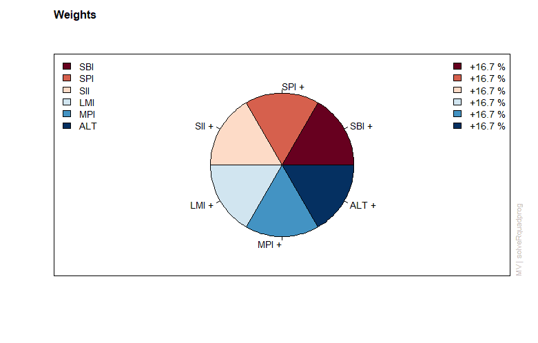
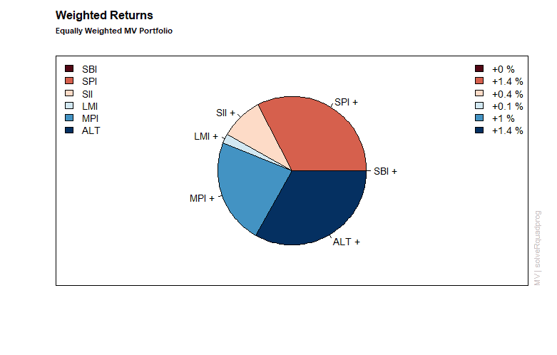
Portfolio Weights:
SBI SPI SII LMI MPI ALT
0.1667 0.1667 0.1667 0.1667 0.1667 0.1667
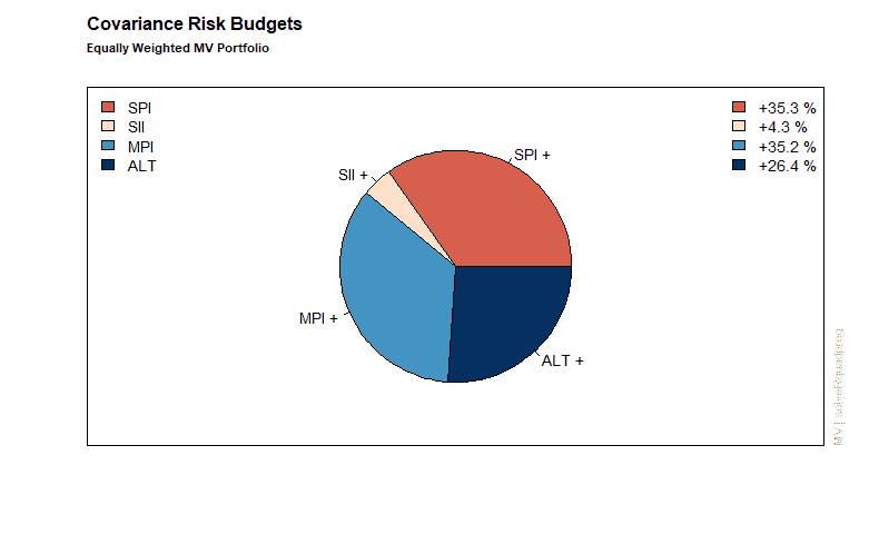
Covariance Risk Budgets:
SBI SPI SII LMI MPI ALT
-0.0039 0.3526 0.0431 -0.0079 0.3523 0.2638
Target Returns and Risks:
mean Cov CVaR VaR
0.0431 0.3198 0.7771 0.4472
Next, we display the results form the equal weights portfolio including the assignment of weights and the attribution of returns and risk.
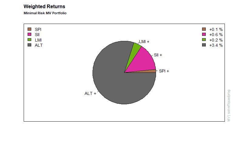
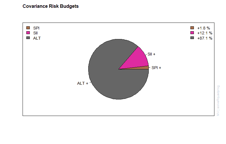
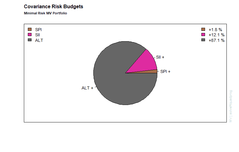
Minimum risk efficient portfolio
We calculate the efficient mean-variance portfolio with the lowest risk for a given return. With the function portfolioSpec() we define a target return and optimize our portfolio.
>library("fPortfolio")
>minriskSpec <- portfolioSpec()
>targetReturn <- getTargetReturn(ewPortfolio@portfolio)["mean"]
>setTargetReturn(minriskSpec) <- targetReturn
>minriskPortfolio <- efficientPortfolio(
+     data = lppData,
+     spec = minriskSpec,
+     constraints = "LongOnly")
> print(minriskPortfolio)

Title:
 MV Efficient Portfolio
 Estimator:         covEstimator
 Solver:            solveRquadprog
 Optimize:          minRisk
 Constraints:       LongOnly

Portfolio Weights:
   SBI    SPI    SII    LMI    MPI    ALT
0.0000 0.0086 0.2543 0.3358 0.0000 0.4013

Covariance Risk Budgets:
    SBI     SPI     SII     LMI     MPI     ALT
 0.0000  0.0184  0.1205 -0.0100  0.0000  0.8711

Target Returns and Risks:
  mean    Cov   CVaR    VaR
0.0431 0.2451 0.5303 0.3412
Weights and plots are generated as follows.
>col <- qualiPalette(ncol(lppData), "Dark2")
>col <- qualiPalette(ncol(lppData), "Dark2")
>mtext(text = "Minimal Risk MV Portfolio", side = 3, line = 1.5,
+       font = 2, cex = 0.7, adj = 0)
Error in mtext(text = "Minimal Risk MV Portfolio", side = 3, line = 1.5,  :
  plot.new has not been called yet
>weightedReturnsPie(minriskPortfolio, radius = 0.7, col = col)
>mtext(text = "Minimal Risk MV Portfolio", side = 3, line = 1.5,
+       font = 2, cex = 0.7, adj = 0)
>covRiskBudgetsPie(minriskPortfolio, radius = 0.7, col = col)
>mtext(text = "Minimal Risk MV Portfolio", side = 3, line = 1.5,
+       font = 2, cex = 0.7, adj = 0)
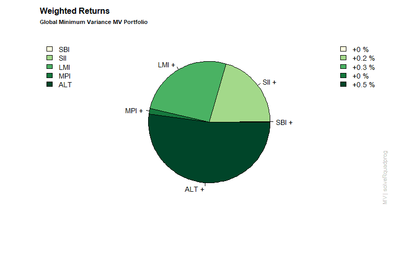
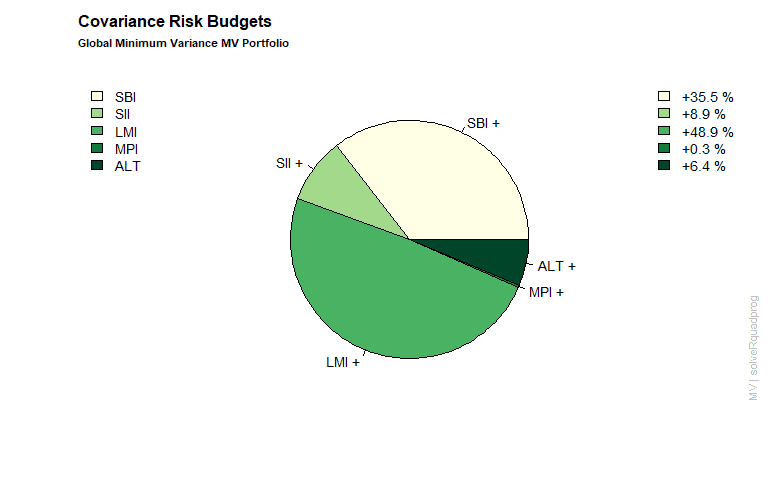
Global minimum variance portfolio
This portfolio finds the best asset allocation with the lowest possible return variance (minimum risk).
>globminSpec <- portfolioSpec()
>globminPortfolio <- minvariancePortfolio(
+     data = lppData,
+     spec = globminSpec,
+     constraints = "LongOnly")
>print(globminPortfolio)

Title:
 MV Minimum Variance Portfolio
 Estimator:         covEstimator
 Solver:            solveRquadprog
 Optimize:          minRisk
 Constraints:       LongOnly

Portfolio Weights:
   SBI    SPI    SII    LMI    MPI    ALT
0.3555 0.0000 0.0890 0.4893 0.0026 0.0636

Covariance Risk Budgets:
   SBI    SPI    SII    LMI    MPI    ALT
0.3555 0.0000 0.0890 0.4893 0.0026 0.0636

Target Returns and Risks:
  mean    Cov   CVaR    VaR
0.0105 0.0986 0.2020 0.1558
In our final step we generate the plots for the global minimum mean-variance portfolio.
>col <- seqPalette(ncol(lppData), "YlGn")
>weightsPie(globminPortfolio, box = FALSE, col = col)
>mtext(text = "Global Minimum Variance MV Portfolio", side = 3,
line = 1.5, font = 2, cex = 0.7, adj = 0)
>weightedReturnsPie(globminPortfolio, box = FALSE, col = col)
>mtext(text = "Global Minimum Variance MV Portfolio", side = 3,
line = 1.5, font = 2, cex = 0.7, adj = 0)
>covRiskBudgetsPie(globminPortfolio, box = FALSE, col = col)
>mtext(text = "Global Minimum Variance MV Portfolio", side = 3,
line = 1.5, font = 2, cex = 0.7, adj = 0)
Case study portfolio optimization
For our real world example we are going to optimize a portfolio of 30 stocks as given in the Dow Jones Index. First we need to load our data set which can be found in the fBasics package.
>djiData <- as.timeSeries(DowJones30)
>djiData.ret <- 100 * returns(djiData)
>colnames(djiData)
 [1] "AA"   "AXP"  "T"    "BA"   "CAT"  "C"    "KO"   "DD"   "EK"   "XOM"  "GE"   "GM"   "HWP"
[14] "HD"   "HON"  "INTC" "IBM"  "IP"   "JPM"  "JNJ"  "MCD"  "MRK"  "MSFT" "MMM"  "MO"   "PG"
[27] "SBC"  "UTX"  "WMT"  "DIS"
>c(start(djiData), end(djiData))
GMT
[1] [1990-12-31] [2001-01-02]
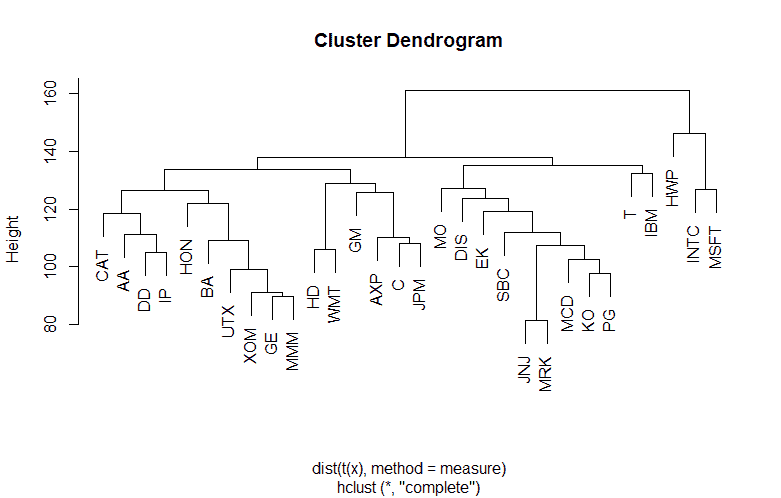
We explore the returns series, investigate pairwise dependencies and the distributional properties from a star plot. With hierarchical clustering and PCA analysis we can find out on whether the stocks are similar or not. To investigate all of these properties we can plot the data and visualize the dependencies with the following code.
>library(fPortfolio)
>for (i in 1:3) plot(djiData.ret[, (10 * i - 9):(10 * i)])
>for (i in 1:3) plot(djiData[, (10 * i - 9):(10 * i)])
>assetsCorImagePlot(djiData.ret)
>plot(assetsSelect(djiData.ret))
>assetsCorEigenPlot(djiData.ret)
Output:


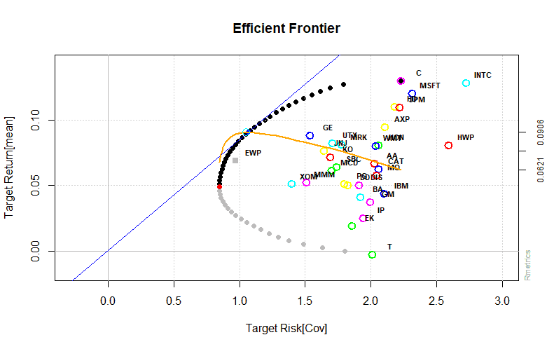
Applying the mean-variance portfolio approach we can find the optimal weights for a long only MV portfolio.
To find the optimal weights for a group-constrained MV portfolio equity clustering is performed. The data is grouped into 5 clusters. A maximum of 50% is invested in each cluster. Clustering is one of the most common exploratory data analysis techniques used to get an intuition about the structure of the data. For our example we use the k-means algorithm. The algorithms modus operandi is to try and make the intra-cluster data points as similar as possible while also keeping the clusters as different (far) as possible. It assigns data points to a cluster such that the sum of the squared distance between the data points and the cluster’s arithmetic mean of all the data points that belong to that cluster is at the minimum. Less variation within clusters means a higher degree of similarity between the data points within the same cluster.
>selection <- assetsSelect(djiData.ret, method = "kmeans")
>cluster <- selection$cluster
>cluster[cluster == 1]
AXP C HD JPM WMT
1 1 1 1 1
>cluster[cluster == 2]
INTC MSFT
2 2
>cluster[cluster == 3]
HWP IBM
3 3
>cluster[cluster == 4]
AA BA CAT DD GM HON IP MMM UTX
4 4 4 4 4 4 4 4 4
>cluster[cluster == 5]
T KO EK XOM GE JNJ MCD MRK MO PG SBC DIS
5 5 5 5 5 5 5 5 5 5 5 5
>constraints <- c(
+ 'maxsumW[c("BA","DD","EK","XOM","GM","HON","MMM","UTX")] = 0.30',
+ 'maxsumW[c(T","KO","GE","HD","JNJ","MCD","MRK","MO","PG","SBC","WMT","DIS")] = 0.30',
+ 'maxsumW[c(AXP","C","JPM")] = 0.30',
+ 'maxsumW[c(AA","CAT","IP")] = 0.30',
+ 'maxsumW[c(HWP","INTC","IBM","MSFT")] = 0.30')
>djiSpec <- portfolioSpec()
>setNFrontierPoints(djiSpec) <- 25
>setEstimator(djiSpec) <- "shrinkEstimator"
>djiFrontier <- portfolioFrontier(djiData.ret, djiSpec)
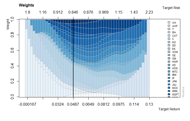
>col = seqPalette(30, "YlOrRd")
>weightsPlot(djiFrontier, col = col)
Output:
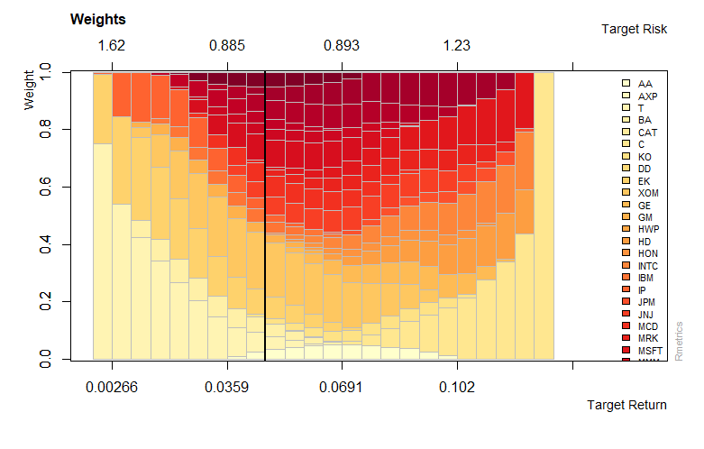
The graph shows the mean-variance frontier for the Dow Jones Index. By using the shrinkage estimator and by computing the weights along the frontier we estimate the covariance matrix.
Mean-CVar portfolio optimization
Portfolio optimization is one of the most important problems from the past that has attracted the attention of investors. In this section we explore mean-CVar portfolio optimization as an alternative approach. Another name for Conditional Value at Risk (CVaR) is Expected Shortfall (ES). Compared to Value at Risk, ES is more sensitive to the tail behavior of the P&L distribution function.
First we select two assets with the smallest and largest returns and divide their range into equidistant parts which determine the target returns for which we try to find efficient portfolios. We compare unlimited short, long-only, box and group constrained efficient frontiers of mean-CVar portfolios.
Unlimited short portfolio
When weights are not restricted we have unlimited short selling. This kind of portfolio cannot be optimized analytically therefore we need to define box constraints with larger lower and upper bounds to circumvent this limitation.
>setNFrontierPoints(shortSpec) <- 5
>setSolver(shortSpec) <- "solveRglpk.CVAR"
>shortFrontier <- portfolioFrontier(data = lppData, spec = shortSpec,
+ constraints = shortConstraints)
>print(shortFrontier)
Title:
CVaR Portfolio Frontier
Estimator: covEstimator
Solver: solveRglpk.CVAR
Optimize: minRisk
Constraints: minW maxW
Portfolio Points: 5 of 5
VaR Alpha: 0.05
Portfolio Weights:
SBI SPI SII LMI MPI ALT
1 0.4257 -0.0242 0.0228 0.5661 0.0913 -0.0816
2 -0.0201 -0.0101 0.1746 0.7134 -0.0752 0.2174
3 -0.3275 -0.0196 0.4318 0.6437 -0.2771 0.5486
4 -0.8113 0.0492 0.5704 0.8687 -0.5273 0.8503
5 -1.6975 0.0753 0.6305 1.5485 -0.6683 1.1115
Covariance Risk Budgets:
SBI SPI SII LMI MPI ALT
1 0.4056 0.0256 0.0062 0.5384 -0.0730 0.0972
2 -0.0080 -0.0173 0.2124 0.4559 -0.1256 0.4825
3 0.0054 -0.0204 0.3674 0.0592 -0.2787 0.8671
4 0.0572 0.0409 0.2901 0.0223 -0.2984 0.8880
5 0.1513 0.0510 0.1966 0.0215 -0.3235 0.9031
Target Returns and Risks:
mean Cov CVaR VaR
1 0.0000 0.1136 0.2329 0.1859
2 0.0215 0.1172 0.2118 0.1733
3 0.0429 0.2109 0.3610 0.2923
4 0.0643 0.3121 0.5570 0.4175
5 0.0858 0.4201 0.7620 0.5745
>setNFrontierPoints(shortSpec) <- 25
>shortFrontier <- portfolioFrontier(data = lppData, spec = shortSpec,
+ constraints = shortConstraints)
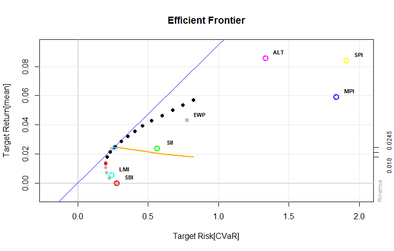
>tailoredFrontierPlot(object = shortFrontier, mText = "Mean-CVaR Portfolio - Short Constraints",
+ risk = "CVaR")
>par(mfrow = c(3, 1), mar = c(3.5, 4, 4, 3) + 0.1)
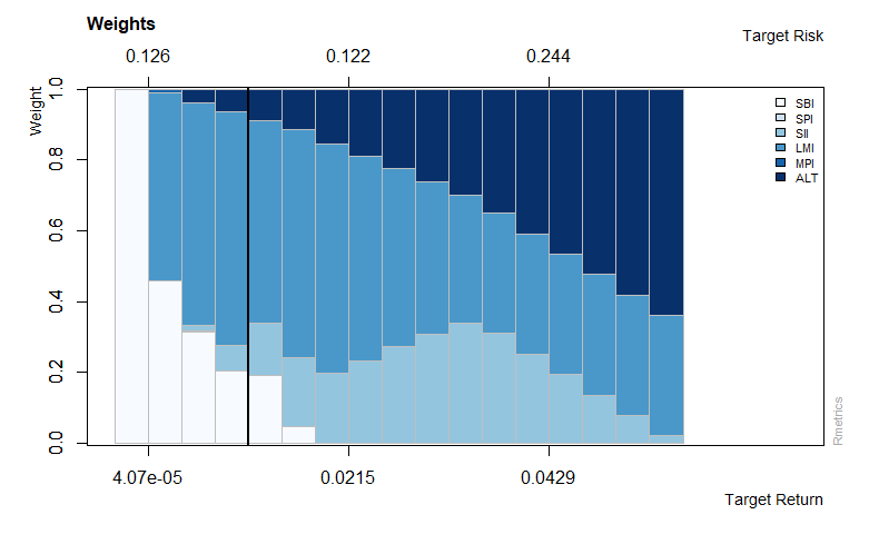
>weightsPlot(shortFrontier)
>text <- "Min-CVaR Portfolio - Short Constrained Portfolio"
>mtext(text, side = 3, line = 3, font = 2, cex = 0.9)
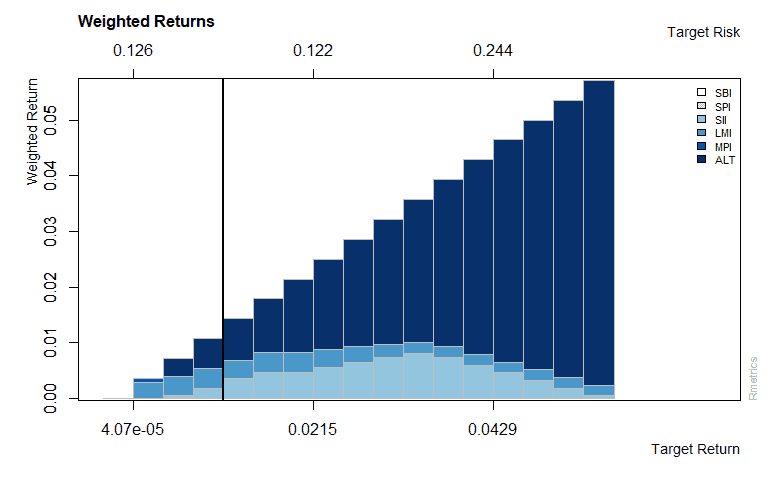
>weightedReturnsPlot(shortFrontier)
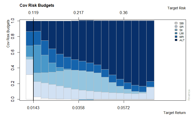
>covRiskBudgetsPlot(shortFrontier)
Output:
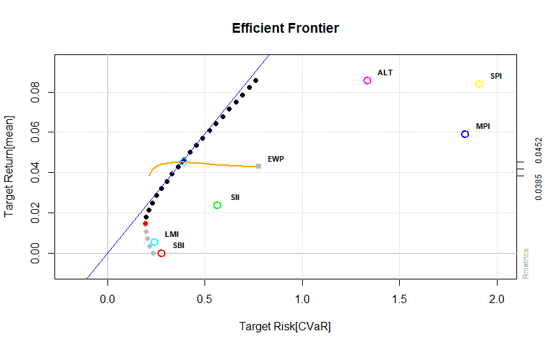
As shown in the graph above risk is lowered through short selling while keeping the same return.
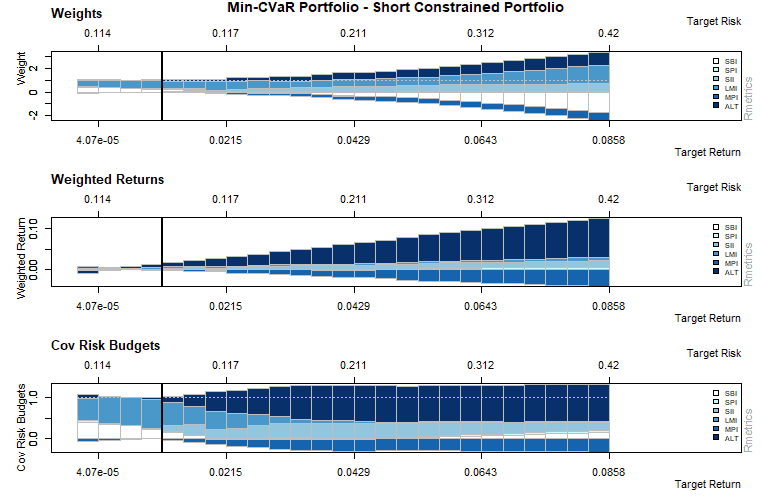
The graph above shows the weighted returns and covariance risk budgets, along the minimum variance locus and the efficient frontier.
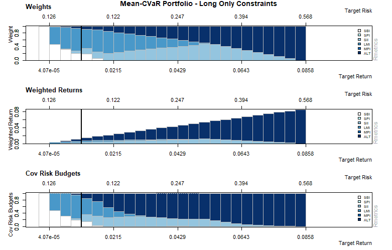
Long only portfolio
For the long only portfolio the weights are bounded between 0 and 1. To compute the efficient frontier of linearly constrained mean-cvar portfolios we can use following functions:
- portfolioFrontier: efficient portfolios on the frontier
- frontierPoints: extracts risk/return frontier points
- frontierPlot: creates an efficient frontier plot
- cmlPoints: adds market portfolio
- cmlLines: adds capital market line
- tangencyPoints: adds tangency portfolio point
- tangencyLines: adds tangency line
- equalWeightsPoints: adds point of equal weights portfolio
- singleAssetPoints: adds points of single asset portfolios
- twoAssetsLines: adds frontiers of two assets portfolios
- sharpeRatioLines: adds Sharpe ratio line
- monteCarloPoints: adds randomly feasible portfolios
- weightsPlot: weights bar plot along the frontier
- weightedReturnsPlot: weighted returns bar plot
- covRiskBudgetsPlot: covariance risk budget bar plot
>lppData <- 100 * LPP2005.RET[, 1:6]
>longSpec <- portfolioSpec()
>setType(longSpec) <- "CVaR"
Solver set to solveRquadprog
setSolver: solveRglpk
>setAlpha(longSpec) <- 0.05
>setNFrontierPoints(longSpec) <- 5
>setSolver(longSpec) <- "solveRglpk.CVAR"
>longFrontier <- portfolioFrontier(data = lppData, spec = longSpec,
+                                   constraints = "LongOnly")
> print(longFrontier)

Title:
 CVaR Portfolio Frontier
 Estimator:         covEstimator
 Solver:            solveRglpk.CVAR
 Optimize:          minRisk
 Constraints:       LongOnly
 Portfolio Points:  5 of 5
 VaR Alpha:         0.05

Portfolio Weights:
     SBI    SPI    SII    LMI    MPI    ALT
1 1.0000 0.0000 0.0000 0.0000 0.0000 0.0000
2 0.0000 0.0000 0.1988 0.6480 0.0000 0.1532
3 0.0000 0.0000 0.3835 0.2385 0.0000 0.3780
4 0.0000 0.0000 0.3464 0.0000 0.0000 0.6536
5 0.0000 0.0000 0.0000 0.0000 0.0000 1.0000

Covariance Risk Budgets:
      SBI     SPI     SII     LMI     MPI     ALT
1  1.0000  0.0000  0.0000  0.0000  0.0000  0.0000
2  0.0000  0.0000  0.2641  0.3126  0.0000  0.4233
3  0.0000  0.0000  0.2432 -0.0101  0.0000  0.7670
4  0.0000  0.0000  0.0884  0.0000  0.0000  0.9116
5  0.0000  0.0000  0.0000  0.0000  0.0000  1.0000

Target Returns and Risks:
    mean    Cov   CVaR    VaR
1 0.0000 0.1261 0.2758 0.2177
2 0.0215 0.1224 0.2313 0.1747
3 0.0429 0.2472 0.5076 0.3337
4 0.0643 0.3941 0.8780 0.5830
5 0.0858 0.5684 1.3343 0.8978
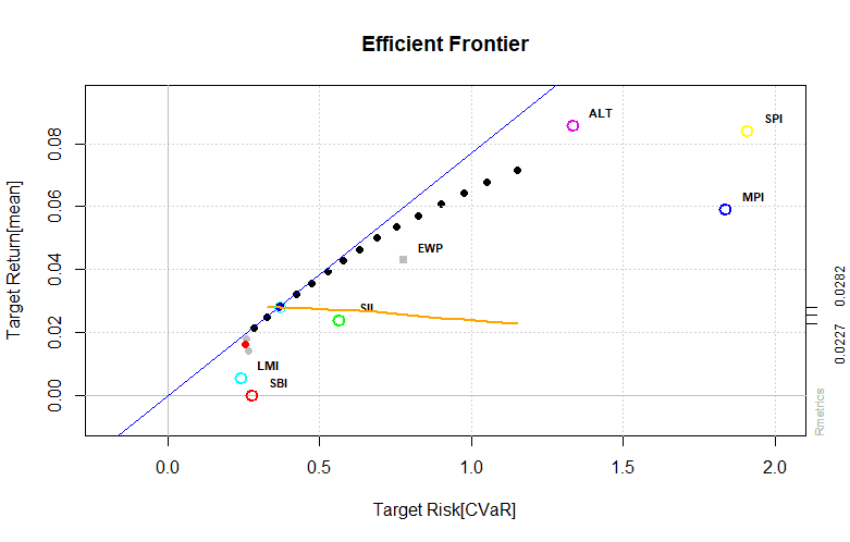
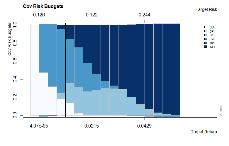
The printout lists portfolio weights, covariance risk budgets and target returns and risks along the efficient frontier. Target returns and risks are sorted starting with the portfolio with the lowest return and ending with the portfolio showing the highest return. By repeating the optimization with 25 points at the frontier we can plot the efficient frontier and the results.
Box constrained portfolio
As the name suggests box-constrained portfolios specify upper and lower bounds on the asset weights.
>boxSpec <- portfolioSpec()
>setType(boxSpec) <- "CVaR"
Solver set to solveRquadprog
setSolver: solveRglpk
>setAlpha(boxSpec) <- 0.05
>setNFrontierPoints(boxSpec) <- 15
>setSolver(boxSpec) <- "solveRglpk.CVAR"
>boxConstraints <- c("minW[1:6]=0.05", "maxW[1:6]=0.66")
>boxFrontier <- portfolioFrontier(data = lppData, spec = boxSpec, constraints = boxConstraints)
>print(boxFrontier)

Title:
 CVaR Portfolio Frontier
 Estimator:         covEstimator
 Solver:            solveRglpk.CVAR
 Optimize:          minRisk
 Constraints:       minW maxW
 Portfolio Points:  5 of 9
 VaR Alpha:         0.05

Portfolio Weights:
     SBI    SPI    SII    LMI    MPI    ALT
1 0.0526 0.0500 0.1370 0.6600 0.0500 0.0504
3 0.0500 0.0500 0.2633 0.4127 0.0500 0.1739
5 0.0500 0.0500 0.4109 0.1463 0.0500 0.2928
7 0.0500 0.0500 0.3378 0.0500 0.0500 0.4622
9 0.0500 0.0501 0.1399 0.0500 0.0500 0.6600

Covariance Risk Budgets:
      SBI     SPI     SII     LMI     MPI     ALT
1  0.0189  0.1945  0.1435  0.3378  0.1742  0.1312
3  0.0023  0.1528  0.2209  0.0248  0.1582  0.4410
5 -0.0017  0.1042  0.2478 -0.0080  0.1136  0.5440
7 -0.0024  0.0823  0.1099 -0.0035  0.0931  0.7206
9 -0.0022  0.0650  0.0182 -0.0031  0.0752  0.8469

Target Returns and Risks:
    mean    Cov   CVaR    VaR
1 0.0184 0.1232 0.2604 0.1913
3 0.0307 0.1838 0.3999 0.2651
5 0.0429 0.2655 0.5787 0.3654
7 0.0552 0.3456 0.7832 0.4818
9 0.0674 0.4388 1.0382 0.6675

Description:
 Thu Jan 28 11:54:41 2021 by user: 1
>setNFrontierPoints(boxSpec) <- 25
>boxFrontier <- portfolioFrontier(data = lppData, spec = boxSpec,
+                                  constraints = boxConstraints)
>tailoredFrontierPlot(object = boxFrontier, mText = "Mean-CVaR Portfolio - Box Constraints",
+                      risk = "CVaR")
>weightsPlot(boxFrontier)
>text <- "Min-CVaR Portfolio - Box Constrained Portfolio"
>mtext(text, side = 3, line = 3, font = 2, cex = 0.9)
>weightedReturnsPlot(boxFrontier)
>covRiskBudgetsPlot(boxFrontier)
Output:
Group constrained portfolio
In a group constrained portfolio the weights of groups are constrained by lower and upper bounds.
> groupSpec <- portfolioSpec()
> setType(groupSpec) <- "CVaR"
Solver set to solveRquadprog
setSolver: solveRglpk
> setAlpha(groupSpec) <- 0.05
> setNFrontierPoints(groupSpec) <- 10
> setSolver(groupSpec) <- "solveRglpk.CVAR"
> groupConstraints <- c("minsumW[c(1,4)]=0.3", "maxsumW[c(2:3,5:6)]=0.66")
> groupFrontier <- portfolioFrontier(data = lppData, spec = groupSpec,
+ constraints = groupConstraints)
> print(groupFrontier)
Title:
CVaR Portfolio Frontier
Estimator: covEstimator
Solver: solveRglpk.CVAR
Optimize: minRisk
Constraints: minsumW maxsumW
Portfolio Points: 5 of 7
VaR Alpha: 0.05
Portfolio Weights:
SBI SPI SII LMI MPI ALT
1 1.0000 0.0000 0.0000 0.0000 0.0000 0.0000
2 0.2440 0.0000 0.0410 0.6574 0.0000 0.0576
4 0.0000 0.0000 0.2744 0.5007 0.0000 0.2249
5 0.0000 0.0000 0.3288 0.3400 0.0000 0.3312
7 0.0000 0.0000 0.0209 0.3400 0.0000 0.6391
Covariance Risk Budgets:
SBI SPI SII LMI MPI ALT
1 1.0000 0.0000 0.0000 0.0000 0.0000 0.0000
2 0.2294 0.0000 0.0218 0.7226 0.0000 0.0263
4 0.0000 0.0000 0.3024 0.0780 0.0000 0.6196
5 0.0000 0.0000 0.2388 -0.0024 0.0000 0.7636
7 0.0000 0.0000 0.0020 -0.0159 0.0000 1.0139
Target Returns and Risks:
mean Cov CVaR VaR
1 0.0000 0.1261 0.2758 0.2177
2 0.0096 0.1012 0.2003 0.1622
4 0.0286 0.1575 0.3076 0.2178
5 0.0381 0.2147 0.4392 0.2783
7 0.0572 0.3559 0.8228 0.5517
> setNFrontierPoints(groupSpec) <- 25
> groupFrontier <- portfolioFrontier(data = lppData, spec = groupSpec,
+ constraints = groupConstraints)
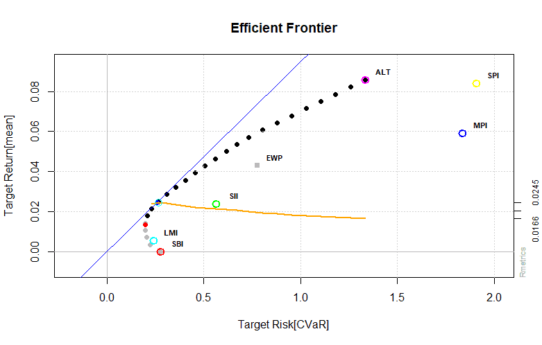
> tailoredFrontierPlot(object = groupFrontier, mText = "Mean-CVaR Portfolio - Group Constraints",
+ risk = "CVaR")
> weightsPlot(groupFrontier)
> text <- "Min-CVaR Portfolio - Group Constrained Portfolio"
> mtext(text, side = 3, line = 3, font = 2, cex = 0.9)
> weightedReturnsPlot(groupFrontier)
> covRiskBudgetsPlot(groupFrontier)
Output:
Portfolio backtesting
For backtesting a portfolio it is common practice to test your strategy performance over a long time frame that encompasses different types of market conditions. We use the S4 object class fPFOLIOBACKTEST to run our backtest. The object of class fPFOLIOBACKTEST has four slots:
@windows
a list, setting the windows function that defines the rolling windows, and the set of window specific parameters params. E.g The window horizon is set as a parameter horizon = "24m"
@strategy
a list, setting the portfolio strategy to implement during the backtest, and any strategy specific parameters are found in params.
@smoother
a list, specifying the smoothing style, given as a smoother function, and any smoother specific parameters are stored in the list params.
@messages
a list, any messages collected during the backtest
We can set the backtest settings with the function portfolioBacktest().
>library(fPortfolio)
>showClass("fPFOLIOBACKTEST")
Class "fPFOLIOBACKTEST" [package "fPortfolio"]

Slots:

Name:   windows strategy smoother messages
Class:     list     list     list     list
>formals(portfolioBacktest)
$windows
list(windows = "equidistWindows", params = list(horizon = "12m"))

$strategy
list(strategy = "tangencyStrategy", params = list())

$smoother
list(smoother = "emaSmoother", params = list(doubleSmoothing = TRUE,
    lambda = "3m", skip = 0, initialWeights = NULL))

$messages
list()
The above code shows you the default settings for the portfolioBacktest() function consisting of a tangency portfolio strategy, equidistant windows with a horizon of 12 months and a double exponential moving average smoother. To create a new backtest function and print the structure for the default settings we can do the following:
>backtest <- portfolioBacktest()
>str(backtest, width = 65, strict.width = "cut")
Formal class 'fPFOLIOBACKTEST' [package "fPortfolio"] with 4 sl..
  ..@ windows :List of 2
  .. ..$ windows: chr "equidistWindows"
  .. ..$ params :List of 1
  .. .. ..$ horizon: chr "12m"
  ..@ strategy:List of 2
  .. ..$ strategy: chr "tangencyStrategy"
  .. ..$ params  : list()
  ..@ smoother:List of 2
  .. ..$ smoother: chr "emaSmoother"
  .. ..$ params  :List of 4
  .. .. ..$ doubleSmoothing: logi TRUE
  .. .. ..$ lambda         : chr "3m"
  .. .. ..$ skip           : num 0
  .. .. ..$ initialWeights : NULL
  ..@ messages: list()
@windows slot:
The slot consists of two named entries. The rolling windows function defines the backtest windows and the second slot named params holds the parameters, for example the horizon of windows.
@windows SLOT OF AN fPFOLIOBACKTEST OBJECT extractor functions:
getWindows: gets windows slot
getWindowsFun: gets windows function
getWindowsParams: gets windows specific parameters
getWindowsHorizon: gets windows horizon
With the constructor functions we can modify the settings for the portfolio backtest specifications.
Constructor Functions
setWindowsFun: sets the name of the windows function
setWindowsParams: sets parameters for the windows function
setWindowsHorizon: sets the windows horizon measured in months
The default rolling windows can be inspected with following code.
>defaultBacktest <- portfolioBacktest()
>getWindowsFun(defaultBacktest)
[1] "equidistWindows"
>getWindowsParams(defaultBacktest)
$horizon
[1] "12m"

> getWindowsHorizon(defaultBacktest)
[1] "12m"
> args(equidistWindows)
function (data, backtest = portfolioBacktest())
NULL
> equidistWindows
function (data, backtest = portfolioBacktest())
{
    horizon = getWindowsHorizon(backtest)
    ans = rollingWindows(x = data, period = horizon, by = "1m")
    ans
}
<bytecode: 0x000001ff58ed37b8>
<environment: namespace:fPortfolio>
The function getWindowsHorizton() extracts the horizon which is the length of the windows. The function rollingWindows() creates the windows returning a list with two entries named from and to. Both of the list entries give the start and end dates of the whole series.
>swxData <- 100 * SWX.RET
>swxBacktest <- portfolioBacktest()
>setWindowsHorizon(swxBacktest) <- "24m"
>equidistWindows(data = swxData, backtest = swxBacktest)
$from
GMT
 [1] [2000-01-01] [2000-02-01] [2000-03-01] [2000-04-01] [2000-05-01] [2000-06-01] [2000-07-01]
 [8] [2000-08-01] [2000-09-01] [2000-10-01] [2000-11-01] [2000-12-01] [2001-01-01] [2001-02-01]
[15] [2001-03-01] [2001-04-01] [2001-05-01] [2001-06-01] [2001-07-01] [2001-08-01] [2001-09-01]
[22] [2001-10-01] [2001-11-01] [2001-12-01] [2002-01-01] [2002-02-01] [2002-03-01] [2002-04-01]
[29] [2002-05-01] [2002-06-01] [2002-07-01] [2002-08-01] [2002-09-01] [2002-10-01] [2002-11-01]
[36] [2002-12-01] [2003-01-01] [2003-02-01] [2003-03-01] [2003-04-01] [2003-05-01] [2003-06-01]
[43] [2003-07-01] [2003-08-01] [2003-09-01] [2003-10-01] [2003-11-01] [2003-12-01] [2004-01-01]
[50] [2004-02-01] [2004-03-01] [2004-04-01] [2004-05-01] [2004-06-01] [2004-07-01] [2004-08-01]
[57] [2004-09-01] [2004-10-01] [2004-11-01] [2004-12-01] [2005-01-01] [2005-02-01] [2005-03-01]
[64] [2005-04-01] [2005-05-01] [2005-06-01]

$to
GMT
 [1] [2001-12-31] [2002-01-31] [2002-02-28] [2002-03-31] [2002-04-30] [2002-05-31] [2002-06-30]
 [8] [2002-07-31] [2002-08-31] [2002-09-30] [2002-10-31] [2002-11-30] [2002-12-31] [2003-01-31]
[15] [2003-02-28] [2003-03-31] [2003-04-30] [2003-05-31] [2003-06-30] [2003-07-31] [2003-08-31]
[22] [2003-09-30] [2003-10-31] [2003-11-30] [2003-12-31] [2004-01-31] [2004-02-29] [2004-03-31]
[29] [2004-04-30] [2004-05-31] [2004-06-30] [2004-07-31] [2004-08-31] [2004-09-30] [2004-10-31]
[36] [2004-11-30] [2004-12-31] [2005-01-31] [2005-02-28] [2005-03-31] [2005-04-30] [2005-05-31]
[43] [2005-06-30] [2005-07-31] [2005-08-31] [2005-09-30] [2005-10-31] [2005-11-30] [2005-12-31]
[50] [2006-01-31] [2006-02-28] [2006-03-31] [2006-04-30] [2006-05-31] [2006-06-30] [2006-07-31]
[57] [2006-08-31] [2006-09-30] [2006-10-31] [2006-11-30] [2006-12-31] [2007-01-31] [2007-02-28]
[64] [2007-03-31] [2007-04-30] [2007-05-31]

attr(,"control")
attr(,"control")$start
GMT
[1] [2000-01-04]

attr(,"control")$end
GMT
[1] [2007-05-08]

attr(,"control")$period
[1] "24m"

attr(,"control")$by
[1] "1m"
To modify rolling window parameters we do the following.
>setWindowsHorizon(backtest) <- "24m"
>getWindowsParams(backtest)
$horizon
[1] "24m"
@strategy slot:
The @strategy slot consists of two named entries. The strategy entry holds the name of the strategy function that defines the portfolio strategy we want to backtest and the params entry holds the strategy parameters.
@strategy SLOT of an fPFOLIOBACKTEST object extractor functions:
getStrategy: gets strategy slot
getStrategyFun: gets the name of the strategy function
getStrategyParams: gets strategy specific parameters
Constructor functions:
setStrategyFun: sets the name of the strategy function
setStrategyParams: sets strategy specific parameters
We can inspect default portfolio strategy settingsby suing tangencyStrategy.
>args(tangencyStrategy)
function (data, spec = portfolioSpec(), constraints = "LongOnly",
    backtest = portfolioBacktest())
NULL

#The following example invests in a strategy with the highest #Sharpe ratio, if such a portfolio is not found the minimum- #variance portfolio is taken instead.
>tangencyStrategy
function (data, spec = portfolioSpec(), constraints = "LongOnly",
    backtest = portfolioBacktest())
{
    strategyPortfolio <- try(tangencyPortfolio(data, spec, constraints))
    if (class(strategyPortfolio) == "try-error") {
        strategyPortfolio <- minvariancePortfolio(data, spec,
            constraints)
    }
    strategyPortfolio
}
<bytecode: 0x000001ff54cdb1c0>
<environment: namespace:fPortfolio>
@smoother slot:
This is a list with two named entries. The entry named smoother holds the name of the smoother function. The function defines the backtest function to smooth the weights over time. The params entry holds the required parameters for the smoother function.
We can inspect the default smoother function with following code.
>args(emaSmoother)
function (weights, spec, backtest)
NULL
> emaSmoother
function (weights, spec, backtest)
{
    ema <- function(x, lambda) {
        x = as.vector(x)
        lambda = 2/(lambda + 1)
        xlam = x * lambda
        xlam[1] = x[1]
        ema = filter(xlam, filter = (1 - lambda), method = "rec")
        ema[is.na(ema)] <- 0
        as.numeric(ema)
    }
    lambda <- getSmootherLambda(backtest)
    lambdaLength <- as.numeric(substr(lambda, 1, nchar(lambda) -
        1))
    lambdaUnit <- substr(lambda, nchar(lambda), nchar(lambda))
    stopifnot(lambdaUnit == "m")
    lambda <- lambdaLength
    nAssets <- ncol(weights)
    initialWeights = getSmootherInitialWeights(backtest)
    if (!is.null(initialWeights))
        weights[1, ] = initialWeights
    smoothWeights1 = NULL
    for (i in 1:nAssets) {
        EMA <- ema(weights[, i], lambda = lambda)
        smoothWeights1 <- cbind(smoothWeights1, EMA)
    }
    doubleSmooth <- getSmootherDoubleSmoothing(backtest)
    if (doubleSmooth) {
        smoothWeights = NULL
        for (i in 1:nAssets) {
            EMA <- ema(smoothWeights1[, i], lambda = lambda)
            smoothWeights = cbind(smoothWeights, EMA)
        }
    }
    else {
        smoothWeights <- smoothWeights1
    }
    rownames(smoothWeights) <- rownames(weights)
    colnames(smoothWeights) <- colnames(weights)
    smoothWeights
}
<bytecode: 0x000001ff549db078>
<environment: namespace:fPortfolio>
With the setSmoother functions we can modify the control parameters.
#Change single smoothing type
>setSmootherDoubleSmoothing(backtest) <- FALSE
#Modify smoother's decay length
> setSmootherLambda(backtest) <- "12m"
#Start rebalancing 12 months after start date
> setSmootherSkip(backtest) <- "12m"
#Use equal weights as starting points
> nAssets <- 5
> setSmootherInitialWeights(backtest) <- rep(1/nAssets, nAssets)
#Check your settings after making changes
> getSmootherParams(backtest)
$doubleSmoothing
[1] FALSE

$lambda
[1] "12m"

$skip
[1] "12m"

$initialWeights
[1] 0.2 0.2 0.2 0.2 0.2
Backtesting sector rotation portfolio
The SPI data is used for the purpose of this backtest. The swiss performance index is comprised of nine sectors: finance, technology, materials, consumer goods, industrials, health care, consumer services, utilities and telecommunications. The strategy uses a fixed rolling window of 12 months shifted in monthly intervals. Portfolio optimization is done via the mean-variance Markowitz method. The first thing we need to do is specify the portfolio data for the specification, for the constraints and for the portfolio backtest.
>library(fPortfolio)
>colnames(SPISECTOR.RET)
 [1] "SPI"  "BASI" "INDU" "CONG" "HLTH" "CONS" "TELE" "UTIL" "FINA" "TECH"
>spiData <- SPISECTOR.RET
>spiSpec <- portfolioSpec()
>spiConstraints <- "LongOnly"
>spiBacktest <- portfolioBacktest()

#Specify assets for backtesting
>spiFormula <- SPI ~ BASI + INDU + CONG + HLTH + CONS + TELE +
+     UTIL + FINA + TECH

#Optimize rolling portfolios and run backtests
>spiPortfolios <- portfolioBacktesting(formula = spiFormula,
+                                       data = spiData, spec = spiSpec, constraints = spiConstraints,
+                                       backtest = spiBacktest, trace = FALSE)

#Weights of first 12 months are rebalanced on a monthly basis
>Weights <- round(100 * spiPortfolios$weights, 2)[1:12, ]
>Weights
           BASI INDU  CONG HLTH CONS TELE   UTIL  FINA TECH
2000-12-31    0    0 48.08    0    0    0  27.54 16.06 8.33
2001-01-31    0    0 22.25    0    0    0  28.62 49.13 0.00
2001-02-28    0    0 31.15    0    0    0  32.80 36.05 0.00
2001-03-31    0    0 51.92    0    0    0  48.08  0.00 0.00
2001-04-30    0    0 39.77    0    0    0  46.70 13.53 0.00
2001-05-31    0    0 35.16    0    0    0  64.68  0.16 0.00
2001-06-30    0    0 47.84    0    0    0  52.16  0.00 0.00
2001-07-31    0    0 27.19    0    0    0  72.81  0.00 0.00
2001-08-31    0    0  0.00    0    0    0 100.00  0.00 0.00
2001-09-30    0    0  0.00    0    0  100   0.00  0.00 0.00
2001-10-31    0    0  0.00    0    0  100   0.00  0.00 0.00
2001-11-30    0    0  0.00    0    0  100   0.00  0.00 0.00
To reduce the costs of rebalancing to often we set the smoothing parameter lambda to 12 months. This way we increase the smoothing effect.
>setSmootherLambda(spiPortfolios$backtest) <- "12m"
>spiSmoothPortfolios <- portfolioSmoothing(object = spiPortfolios,
+                                           trace = FALSE)
>smoothWeights <- round(100 * spiSmoothPortfolios$smoothWeights,
+                        2)[1:12, ]
>smoothWeights
           BASI INDU  CONG HLTH CONS  TELE  UTIL  FINA TECH
2000-12-31    0    0 48.08    0    0  0.00 27.54 16.06 8.33
2001-01-31    0    0 47.47    0    0  0.00 27.56 16.84 8.13
2001-02-28    0    0 46.64    0    0  0.00 27.70 17.86 7.80
2001-03-31    0    0 46.18    0    0  0.00 28.29 18.16 7.37
2001-04-30    0    0 45.70    0    0  0.00 29.14 18.27 6.89
2001-05-31    0    0 45.10    0    0  0.00 30.59 17.92 6.39
2001-06-30    0    0 44.74    0    0  0.00 32.15 17.24 5.88
2001-07-31    0    0 44.06    0    0  0.00 34.22 16.35 5.37
2001-08-31    0    0 42.54    0    0  0.00 37.26 15.32 4.88
2001-09-30    0    0 40.44    0    0  2.37 38.55 14.23 4.41
2001-10-31    0    0 37.98    0    0  6.37 38.57 13.11 3.98
2001-11-30    0    0 35.32    0    0 11.46 37.67 11.99 3.57
Plot backtests
>backtestPlot(spiSmoothPortfolios, cex = 0.6, font = 1, family = "mono")

#
>netPerformance(spiSmoothPortfolios)

Net Performance % to 2008-10-31:
          1 mth 3 mths 6 mths  1 yr 3 yrs 5 yrs 3 yrs p.a. 5 yrs p.a.
Portfolio -0.21  -0.25  -0.31 -0.44 -0.26  0.49      -0.09       0.10
Benchmark -0.13  -0.17  -0.22 -0.38 -0.29  0.29      -0.10       0.06


Net Performance % Calendar Year:
           2001  2002 2003 2004 2005 2006 2007   YTD Total
Portfolio -0.10 -0.09 0.25 0.25 0.22 0.29 0.05 -0.39  0.48
Benchmark -0.25 -0.30 0.20 0.07 0.30 0.19 0.00 -0.32 -0.11
Output:
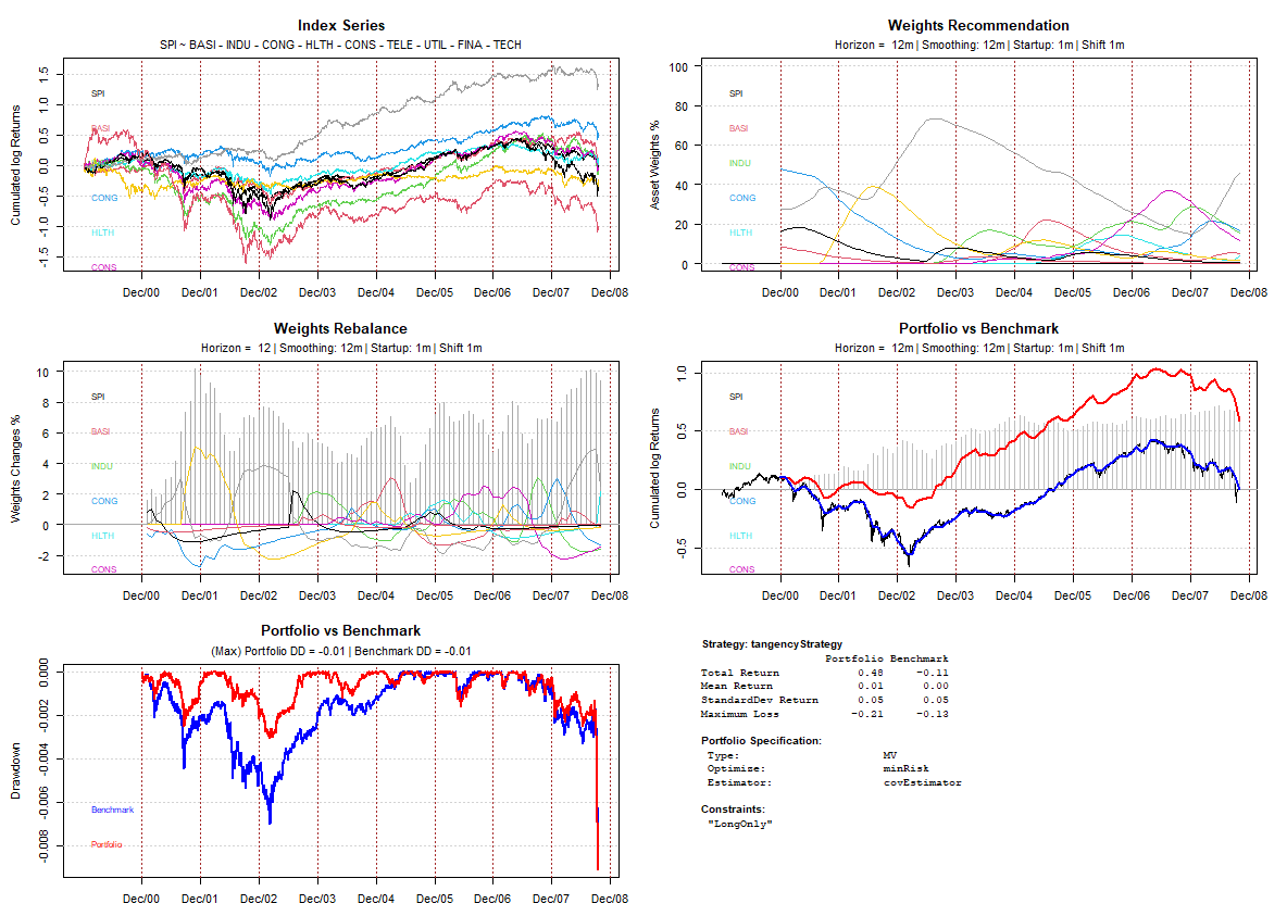
As shown in above graph if we had started the strategy in January 2001 the total portfolio return would have been 79.60%. During 2002 and 2003 when the market was on a downward trend the portfolio was able to absorb losses better than the benchmark. The amount of rebalancing see graph “Weights Rebalance” was also reasonable with a per month rebalancing of around 8%. Weights are smoothed with a double EMA smoother with a time decay of 6 months. The total return for the time frame tested is 48% for our portfolio vs -11% for the benchmark.
What to do next
If you made it through the end of this tutorial and you still don’t have enough we recommend you read the following books to gain a deeper understanding on the theoretical background of portfolio optimization.
Robust Portfolio Optimization and Management
Quantitative Equity Portfolio Management: Modern Techniques and Applications
Advances in Active Portfolio Management: New Developments in Quantitative Investing
————
References
Bacon, C. R. (2008). Practical Portfolio Performance Measurement and
Attribution (2 ed.). JohnWiley & Sons.
DeMiguel, V.; Garlappi, L.; and Uppal, R. (2009) . “Optimal versus Naive Diversification: How Inefficient Is the 1/N Portfolio Strategy?”. The Review of Financial Studies, pp. 1915—195.
DiethelmWürtz, Tobias Setz,William Chen, Yohan Chalabi, Andrew Ellis (2010). “Portfolio Optimization with R/Rmetrics”.
Guofu Zhou (2008) “On the Fundamental Law of Active Portfolio Management: What Happens If Our Estimates Are Wrong?” The Journal of Portfolio Management, pp. 26-33
Taleb N.N. (2019). The Statistical Consequences of Fat Tails (Technical Incerto Collection)
Würtz, D. & Chalabi, Y. (2009a). The fPortfolio Package. cran.r-project.org.
Wang, N. &Raftery, A. (2002). Nearest neighbor variance estimation (nnve):
Robust covariance estimation via nearest neighbor cleaning. Journal of
the American Statistical Association, 97, 994–1019.
Spread Trading Sector Index Futures – CME Group – CME Group https://www.cmegroup.com/education/articles-and-reports/spread-trading-sector-index-futures.html