
Build a Trading System using Statistical Methods
Most trading systems utilize indicators as a method of trading strategy design. But before building a trading system using indicators one should ask what do they indicate? The answer to that is that most of the time they are not indicating any information that can be advantageous in building a profitable trading system. The only thing that they can be used for are as noise filters. Some indicators such as the stochastic oscillator refers to the point of a current price in relation to its price range over a period of time which means that the longer price waves are filtered out and the data is displayed in form of a price divergence-convergence in an extreme area. Other trading systems use heuristic methods such as “buy after x bars are higher than the previous highest bar and sell when next bar lower than the previous x lows.” Clearly we are building our system on a limited data range hoping for future prices to repeat in similar fashion in order to keep our rule valid. This indicates a false assumption of consistent repetition of a small range of price patterns. Other trading systems attempt to predict the price movement by using volume. Which is also something that makes a trading system rarely profitable. This is especially true for high frequency trading strategies. A lot of the trading volume generated during the day comes from dark pools which are obligated to report trade data within a time window of 10 seconds. This basically means you are receiving transaction data with a time lag of up to 10 seconds.
The process of trading system design is a process of statistical based price prediction. In this post we will illustrate some basics that show if a certain event can give you the statistical edge to predict future price movements. Once you identify a predictive event it becomes much easier to design a trading system around it.
Our process of designing a trading system starts with identifying price patterns beginning from a specific event. Previous research indicates that there is cycle activity in index futures. The cycle is consistent with the monthly observation that companies make their numbers on a monthly basis (Ehlers, 2013). Since a month consists of 20 trading days we can say that a cycle consists of 10 up and 10 down days (Ehlers, 2013). Therefore we start with the presumption that we want to predict price behavior for the next 10 trading days. Our point of reference is 10 days back in history. Here is the EasyLanguage Code for it:
https://gist.github.com/18182324/00eddb440eff9a97aedbca1455ce600b
The event cycle can be changed to any number depending on the asset you want to analyze. As for our case when an event occurs, the percentage change in prices over the next 10 days is computed. The percentage price is assigned to the variable FuturePrice which is limited between -10% and 10%. After limiting the range, FuturePrice is rescaled to vary from zero to 100. As described by Ehlers (2013) the goal is to accumulate the number of occurrences of a FuturePrice in each of the bins over a time span of 10 years of historical data. The number of occurrences creates a probability distribution function of the prices 10 bars into the future beginning with the occurrence of the event. Another provided measure is center of gravity (CG) which measures the average percentage future price of the probability distribution. As shown in the easylanguage code above, a folder is created on the computer named C:\PDFTest when the last bar on the chart is encountered. The file is then imported into excel to view the probability distribution function by plotting it as a vertical bar chart [how to tutorial for calculating probability distributions in excel]. Here is an example of this process with the complete strategy code (Ehlers, 2013):
https://gist.github.com/18182324/00eddb440eff9a97aedbca1455ce600b
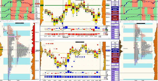
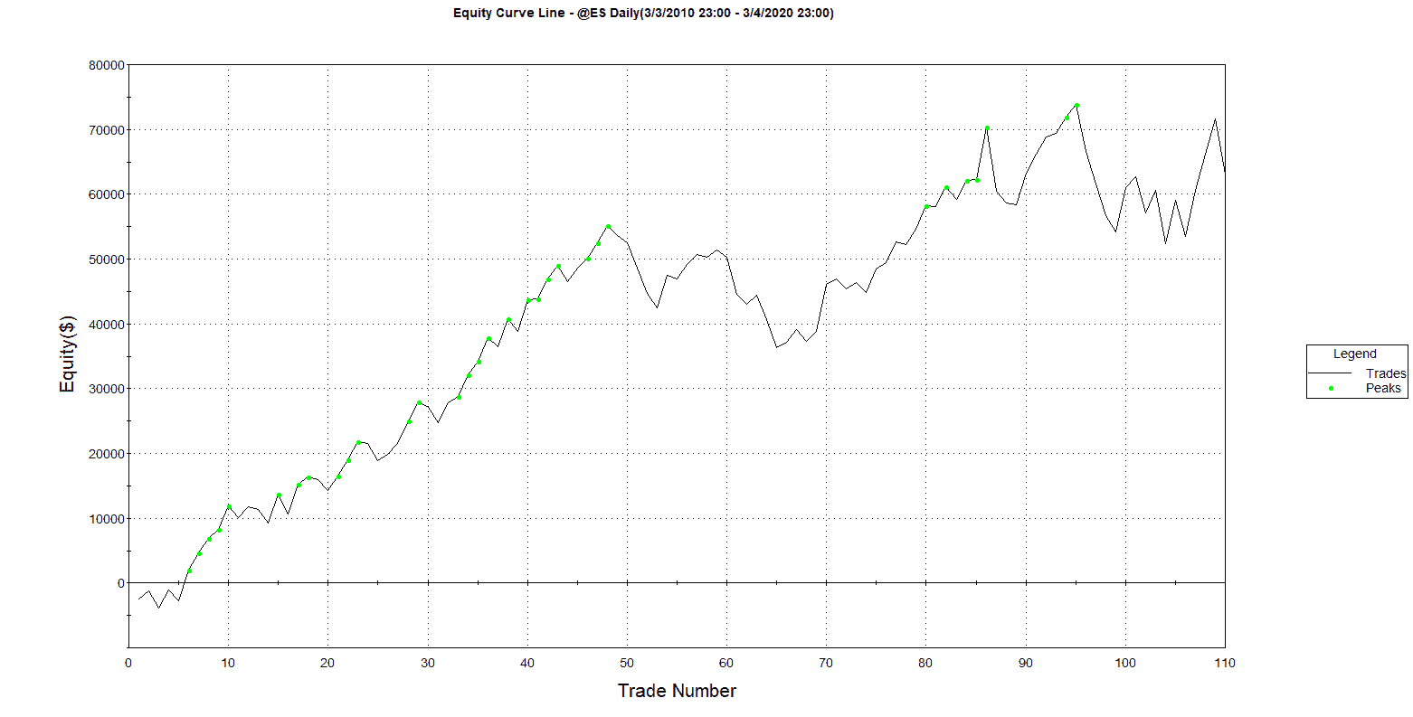
Since we are anticipating the event our trading strategy will enter long when the stochastic crosses a threshold of 0.3 with a stochastic length of 8. After our optimization run the best trading length is found at 14 bars into the future. For simplicity reasons we have set the stop loss at 3.8%. A more effective stop loss strategy could be developed by using more sophisticated money management strategies such as optimal f (Vince, 1992). Applying this strategy to 10 years of data gives us the following equity curve:
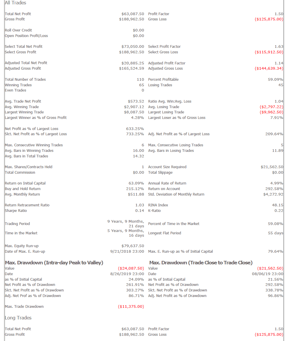
The following performance report gives us a detailed evaluation of the strategy:
The outlined strategy represents a general framework for the development of a trading system based on a statistical approach. The framework is capable of assessing whether a price will increase or decrease over X bars after an event. In our test data we have used daily bars but the framework is applicable to any data granularity.
References:
Ehlers, John F. 2013. Cycle Analytics for Traders, + Downloadable Software: Advanced Technical Trading Concepts. 1 edition. Hoboken, New Jersey: Wiley.
Ralph, Vince. 1992. The Mathematics of Money Management: Risk Analysis Techniques for Traders. Wiley.
If you like our article sign up here for more in-depth research [We publish trading strategies & research using R, Python and EasyLanguage]