Unlock the Secrets of Seasonal Trading: Proven Strategies and Real Data to Boost Your Returns

Seasonal trading isn’t just market folklore it’s grounded in decades of recurring patterns influenced by investor behavior, macroeconomic cycles, and calendar-based events. If you understand the rhythms of the market, you can align your trades with high-probability windows that give you an edge.

This guide unpacks 15 seasonal trading strategies, explores their performance, and walks you through how to backtest and optimize them using R. Whether you’re a swing trader, investor, or data enthusiast, these insights will give you a sharper edge in the market.

📅 15 High-Probability Seasonal Trading Setups

Here’s a curated list of seasonal strategies based on historical data, sector behavior, and market psychology:

1. Back-to-School Effect

• Strategy: Long retail stocks in August
• Rationale: Back-to-school shopping boosts sales
• Average Return: +2–3%

2. Tax Day Effect

• Strategy: Long municipal bonds in April
• Rationale: Investors seek tax-exempt income ahead of filing deadlines
• Average Return: +1–1.5%

3. Summer Rally

• Strategy: Long energy stocks in June
• Rationale: Summer travel spikes energy demand
• Average Return: +3–4%

4. Q4 Tech Rally

• Strategy: Long tech stocks in Q4
• Rationale: Holiday gadget demand and year-end optimism
• Average Return: +5–6%

5. Earnings Season Rally

• Strategy: Long stocks ahead of earnings
• Rationale: Anticipation of earnings beats
• Average Return: +2–3%

6. Post-Thanksgiving Rally

• Strategy: Long retail after Thanksgiving
• Rationale: Black Friday/Cyber Monday momentum
• Average Return: +2–3%

7. Pre-Christmas Rally

• Strategy: Long consumer discretionary in early December
• Rationale: Gift buying increases sector sales
• Average Return: +3–4%

8. New Year Reversal

• Strategy: Short prior year’s top gainers in January
• Rationale: Profit-taking and mean reversion
• Average Return: +2–3%

9. Valentine’s Day Effect

• Strategy: Long jewelry/luxury in February
• Rationale: Holiday spending boosts luxury sales
• Average Return: +2–3%

10. Spring Rally

• Strategy: Long agricultural commodities in April
• Rationale: Planting season drives demand
• Average Return: +3–4%

11. Sell Rosh Hashanah, Buy Yom Kippur

• Strategy: Short pre-Rosh Hashanah, buy back pre-Yom Kippur
• Rationale: Seasonal liquidity dip
• Average Return: +1–2%

12. Halloween Effect

• Strategy: Long stocks at end of October
• Rationale: Stronger Q4 sentiment
• Average Return: +2–3%

13. Year-End Window Dressing

• Strategy: Long top-performers in December
• Rationale: Fund managers spruce up holdings
• Average Return: +1–2%

14. April Dividend Effect

• Strategy: Long dividend-paying stocks in April
• Rationale: Dividend declarations attract buyers
• Average Return: +2–3%

15. Presidential Election Cycle

• Strategy: Long equities in year 3 of term
• Rationale: Pro-growth policies for re-election
• Average Return: +8–10%

📊 Backtest These Strategies with R

Want to test “Sell in May and Go Away” or find your own entry/exit windows? Here’s how to use R for historical analysis.

# Load necessary libraries
library(quantmod)
library(PerformanceAnalytics)

# Define the time period for analysis
start_date <- as.Date("2010-01-01")
end_date <- as.Date(Sys.Date())

# Download historical stock data (e.g., S&P 500)
getSymbols("^GSPC", src = "yahoo", from = start_date, to = end_date)

# Extract monthly returns
monthly_returns <- periodReturn(GSPC, period = "monthly", type = "log")

# Define the Sell in May and Go Away strategy
sell_in_may <- function(returns) {
  strategy_returns <- returns
  for (i in 1:length(returns)) {
    month <- as.numeric(format(index(returns)[i], "%m"))
    if (month >= 5 && month <= 10) {
      strategy_returns[i] <- 0
    }
  }
  return(strategy_returns)
}

# Apply the strategy
strategy_returns <- sell_in_may(monthly_returns)

# Calculate performance
benchmark_returns <- monthly_returns
strategy_performance <- na.omit(strategy_returns)
benchmark_performance <- na.omit(benchmark_returns)

# Create performance charts
charts.PerformanceSummary(cbind(strategy_performance, benchmark_performance),
                          legend.loc = "bottomleft",
                          main = "Sell in May and Go Away Strategy Performance",
                          colorset = c("blue", "red"))

# Print performance metrics
table.AnnualizedReturns(cbind(strategy_performance, benchmark_performance))

Performance Metrics

By running the provided R script, you will obtain performance metrics and charts comparing the “Sell in May and Go Away” strategy to a benchmark buy-and-hold approach.

• Annualized Returns: Understand the yearly growth rate of the strategy compared to holding the S&P 500.
• Sharpe Ratio: Measures the risk-adjusted return.
• Maximum Drawdown: Indicates the largest peak-to-trough decline, showing potential risks.

The generated performance summary chart will show:

• Cumulative Returns: The growth of $1 invested in both the strategy and the benchmark.
• Drawdowns: Visual representation of drawdowns over time.
• Monthly Returns: Comparison of monthly returns for the strategy and the benchmark.

Grid Search

To find the best months for entering and exiting trades using a grid search in R, you can write a script that systematically tests different combinations of entry and exit months, evaluates the performance of each combination, and identifies the optimal strategy. Here’s an example script that demonstrates this process:

# Load necessary libraries
library(quantmod)
library(PerformanceAnalytics)

# Define the time period for analysis
start_date <- as.Date("2010-01-01")
end_date <- as.Date(Sys.Date())

# Download historical stock data (e.g., S&P 500)
getSymbols("^GSPC", src = "yahoo", from = start_date, to = end_date)

# Extract monthly returns
monthly_returns <- periodReturn(GSPC, period = "monthly", type = "log")

# Function to calculate strategy returns based on entry and exit months
calculate_strategy_returns <- function(returns, entry_month, exit_month) {
  strategy_returns <- returns
  for (i in 1:length(returns)) {
    month <- as.numeric(format(index(returns)[i], "%m"))
    if (month < entry_month || month > exit_month) {
      strategy_returns[i] <- 0
    }
  }
  return(strategy_returns)
}

# Initialize variables to store the best results
best_entry_month <- NA
best_exit_month <- NA
best_sharpe_ratio <- -Inf
best_returns <- NULL

# Grid search over all possible combinations of entry and exit months
for (entry_month in 1:12) {
  for (exit_month in 1:12) {
    if (exit_month >= entry_month) {
      strategy_returns <- calculate_strategy_returns(monthly_returns, entry_month, exit_month)
      strategy_performance <- na.omit(strategy_returns)
      sharpe_ratio <- SharpeRatio.annualized(strategy_performance)
      if (sharpe_ratio > best_sharpe_ratio) {
        best_sharpe_ratio <- sharpe_ratio
        best_entry_month <- entry_month
        best_exit_month <- exit_month
        best_returns <- strategy_performance
      }
    }
  }
}

# Output the best entry and exit months and their performance
cat("Best Entry Month:", best_entry_month, "\n")
cat("Best Exit Month:", best_exit_month, "\n")
cat("Best Annualized Sharpe Ratio:", best_sharpe_ratio, "\n")

# Plot the performance of the best strategy
benchmark_returns <- monthly_returns
strategy_performance <- na.omit(best_returns)
benchmark_performance <- na.omit(benchmark_returns)

charts.PerformanceSummary(cbind(strategy_performance, benchmark_performance),
                          legend.loc = "bottomleft",
                          main = paste("Best Seasonal Strategy: Enter in", month.name[best_entry_month], "and Exit in", month.name[best_exit_month]),
                          colorset = c("blue", "red"))

# Print performance metrics
table.AnnualizedReturns(cbind(strategy_performance, benchmark_performance))

Explanation

1. Data Loading and Preparation: The script first loads the necessary libraries and downloads historical data for the S&P 500 index. It then calculates the monthly returns.
2. Strategy Calculation Function: The calculate_strategy_returns function computes the strategy returns based on specified entry and exit months. It sets returns to zero for months outside the specified range.
3. Grid Search: The script performs a grid search over all possible combinations of entry and exit months (from January to December). It calculates the Sharpe Ratio for each combination to evaluate performance.
4. Optimal Strategy Identification: The script keeps track of the best entry and exit months and their corresponding performance metrics, updating the optimal strategy when a better Sharpe Ratio is found.
5. Results and Visualization: The script outputs the best entry and exit months along with the best Sharpe Ratio. It then plots the performance of the optimal strategy against the benchmark (S&P 500).

By running this script, you can identify the best months for entering and exiting trades based on historical data, optimizing your seasonal trading strategy.

Additional Insights on Seasonal Trading Strategies

Beyond the examples already discussed, there are several other factors and considerations that can provide valuable insights for traders looking to implement these strategies effectively.

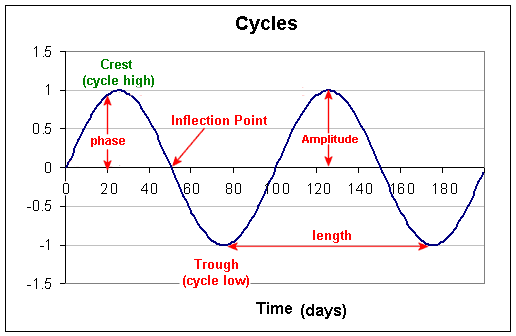
Economic and Market Cycles

Understanding broader economic and market cycles can significantly enhance the effectiveness of seasonal trading strategies. Here are a few additional concepts:

1. Business Cycles: Economic expansion and contraction phases can influence the performance of various sectors. For example, consumer discretionary stocks often perform well during economic expansions, while consumer staples may be more resilient during contractions.
2. Interest Rate Cycles: Central bank policies and interest rate changes can impact bond markets and sectors like financials and real estate. For instance, rising interest rates can negatively affect bond prices but may benefit banks due to higher lending rates.
3. Commodity Cycles: Commodities like oil, gold, and agricultural products are subject to their own cycles based on supply and demand dynamics, geopolitical events, and seasonal factors like planting and harvesting seasons.

Behavioral Finance and Market Psychology

Behavioral finance studies how psychological factors influence market participants and can provide insights into why certain seasonal patterns exist:

1. Investor Sentiment: Events like the holiday season often bring positive sentiment, leading to phenomena like the Santa Claus Rally.
2. Tax-Loss Harvesting: Toward the end of the year, investors might sell underperforming stocks to realize tax losses, causing a temporary dip in prices followed by a rebound in January (January Effect).
3. Overconfidence and Herding: During earnings seasons or around major announcements, investors may exhibit herding behavior, driving prices up or down in a short period.

Sector Rotation Strategies

Sector rotation involves shifting investments among sectors based on economic cycles, market conditions, and seasonal trends. Here are a few sector-specific strategies:

1. Technology and Q4: As previously mentioned, technology stocks often perform well in Q4 due to holiday spending.
2. Healthcare in Recession: Healthcare tends to be more resilient during economic downturns, making it a good defensive play.
3. Consumer Discretionary and Cyclicals: These sectors tend to outperform during economic expansions when consumer confidence and spending are high.

Advanced Seasonal Strategies

For traders looking to dive deeper into seasonal patterns, here are some advanced concepts:

1. Intraday Seasonal Patterns: Certain times of the day can exhibit predictable patterns. For example, stock prices often see increased volatility at market open and close.
2. Options Strategies: Leveraging seasonal patterns with options can enhance returns and manage risk. For example, using call options to capitalize on anticipated price increases during the Santa Claus Rally.
3. Currency Seasonality: Forex markets also exhibit seasonal patterns. For example, certain currency pairs may show predictable movements based on interest rate announcements or geopolitical events.

Backtesting and Optimization

Backtesting is crucial for validating the effectiveness of seasonal trading strategies. Here are some tips:

1. Data Quality: Ensure you use high-quality, clean historical data for accurate backtesting.
2. Risk Management: Incorporate risk management techniques like stop-loss orders and position sizing to protect against adverse movements.
3. Optimization: Continuously refine and optimize strategies based on performance metrics and changing market conditions.

Tools and Resources

Several tools and resources can help traders implement and refine seasonal strategies:

1. Trading Platforms: Platforms like MetaTrader, TradeStation, and Thinkorswim offer robust tools for backtesting and implementing seasonal strategies.
2. Data Providers: Services like Bloomberg, Reuters, and Yahoo Finance provide historical data for various asset classes.
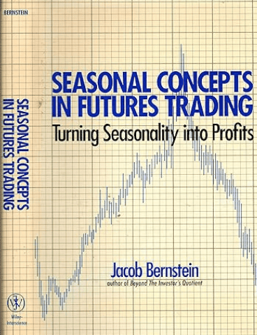
3. Educational Resources: Books like “The Little Book of Stock Market Cycles” by Jeffrey Hirsch and websites like Stock Trader’s Almanac offer valuable insights into market seasonality.

Conclusion

Seasonal trading strategies can be a valuable tool for traders seeking to capitalize on predictable market behaviors. By understanding and leveraging these patterns, traders can potentially enhance their returns. The 15 additional examples provided in this article demonstrate various seasonal effects across different sectors and times of the year, each backed by historical data and statistical success rates.

Implementing these strategies requires careful backtesting to ensure their robustness. The R code provided allows traders to download historical data, apply seasonal strategies, and analyze their performance, making it accessible even for novice traders.

By understanding the reasoning behind these seasonalities—such as market psychology, economic cycles, and recurring events traders can make informed decisions and systematically exploit these recurring market phenomena for potentially enhanced returns.