

Applied Statistics for Futures Markets
In this article we will look at the futures market and how statistical analysis can pave the way for better trading results. What makes the statistical analysis we are going to show you even more important is the fact that you are going to learn how to increase the odds of your trading success in a simple but effective way.
The following tutorial explains how to calculate probability distributions using excel. Price movements are nothing else than the mirror of human emotions consisting of fear and greed. These emotions are reflected in the price movement of an asset and are showing us a repeating pattern. Therefore it is important to know the typical market reactions and price fluctuations of an asset by analyzing and interpreting the statistics behind it. Understanding the statistics behind it can enable us to correctly set stop losses and price targets before we actually enter a trade. The purpose of this guide is to teach you a simple but powerful approach in theoretical statistics.
Let’s start with the definition of a normal distribution. The normal distribution is a probability distribution that associates the normal random variable X with a probability. It is a bell-shaped curve. The curve is wide and short when the standard deviation is large.
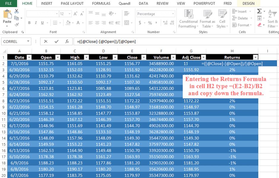
In the following example we are going to look at a statistical analysis of the Russel 2000. Let’s start by downloading the data from Yahoo finance with the ticker symbol ^RUT. When opening yahoo finance browse to the “historical prices” page and download the historical data from 09/10/1987 to 07/05/2016. Now open the data in excel and start calculating the daily returns of the Russel 2000 Index.
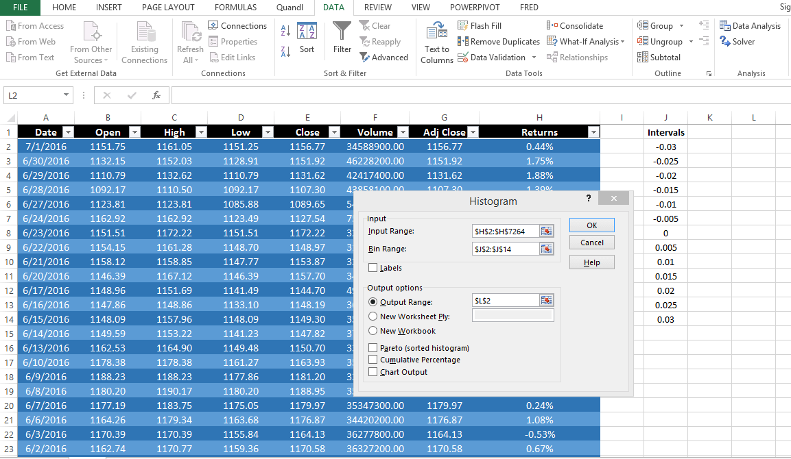
After calculating the daily returns for our time series we are going to analyze the distribution of these returns. We will find out how many up or down days we have for a given % change. First of all we need to choose intervals that will yield meaningful results. The intervals depend on the volatility of the asset we are analyzing. In our case we are going to look at intervals ranging from -3% to 3% in increments of 0.5%. Select cell J2 title it Intervals and write down the intervals. For the next step we use the excel add-in Analysis Toolpak. Locate Data Analysis and click on it to locate Data Analysis Menu. Select Histogram from the list. Select the input range by highlighting cell H2 and press CTRL+SHIFT+DOWN to select all data in the column. Use the same procedure for the bin range by highlighting cell J2 and select all the data in the column. Finally select your output range. It should know look something like this :
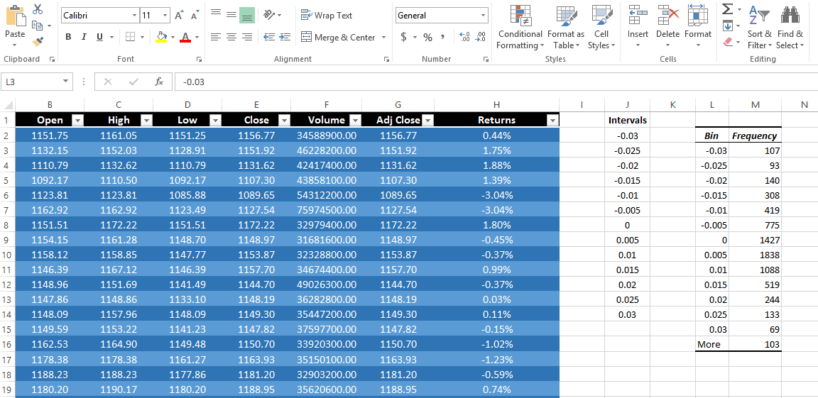
Now highlight the bins and the histogram data cells L3 to M16 and create a histogram. From the list of graph types select 2D option as seen in the screenshot below:

After calculating the daily returns and the probability distributions we can already come to our first conclusions. We can see that the histogram is similar to a normal distribution. In our case we have a fat-tailed distribution which is one of the so-called heavy-tailed statistical distributions that describe the probability of certain events. Fat tails have a sharp bell shape which leads to the term leptokurtosis, another name for a fat-tailed distribution. A probability distribution with fat tails would be one in which moderately extreme outcomes were more likely than you might have expected. In our next step we calculate the descriptive statistics for our time series. In excel select Data Analysis -> Descriptive Statistics . Select the returns Column Highlight H2 (press CTRL+SHIFT+DOWN). Select the output range and check the summary statistics box.


Let’s know discuss our results.

The Median of 0.000950072 is the middle number in our sample. Since the number is positive we can come to the conclusion that we have more positive returns than negative. Given the fact that our median is greater than the mean we can say that the negative returns are of higher magnitude than the positive ones. The mean is our average daily return in our case 0.0325 %. Most advanced economic analysis models study data for skewness and incorporate this into their calculations. Skewness risk is the risk that a model assumes a normal distribution of data, when in fact data is skewed to the left or right of the mean. We have a negative skewness which means that for our distribution of daily returns the negative returns are more extreme than the positive ones. The standard deviation measures the dispersion of our time series from the mean. A high standard deviation means that we have a volatile asset. Standard deviation in this case is the level of volatility of returns measured in percentage terms. Standard deviation is probably used more often than any other measure to gauge risk. Minimum and maximum values show us the change within one trading day. The worst day in the Russel 2000 was a return of-12%. The highest positive return in one trading day was +8.17%. Range tells us the difference between the highest positive trading day and the lowest negative trading day.
Now why is this data so useful? It’s useful for calculating the probability of different returns. We can use the number in our frequency table to create probability values. For example, what is the probability that we will have a certain % change on any given trading day. You can move this analysis and the methods shown one step further by changing the granularity of your data set. Calculate the % change for 1 min time intervals instead of daily data. You can calculate the above statistics and find out what the probabilities are that we have a 1% move up or down within the first hour of a trading day. Calculate the volatility, mean, standard deviation for every granularity and all this can be accomplished by doing what we show you in this post. It’s the basic framework in finding patterns in your data. Let’s move on to the next step. Select cell O4 and type M4/$S$17 and copy the formula down to O17.

In the next step we calculate the cumulative probabilities. In cell P4 type “=O4”. In cell P5 type “P4+O5” and copy the formula down to P17.


After calculating the probabilities we can start concluding a few things. 92.44% of the time the daily returns are 1.5% or less, 54.99% of the time the Russel 2000 Index has had positive returns. Important ? Yes of course, don’t you want to have realistic expectations when you enter a position? Let’s assume the market moves +1.5%(from 1200 to 1218) within the first three hours of the trading day and you go long with a profit target of 1%(entry 1218 and exit at 1230). Our cumulative probability calculations are telling us that the chances for this to happen are 7.56 %(100%-92.44%). Now, what do you think Bud Fox is this a realistic target?
In our next step we are going to calculate the average returns for our time series. First of all add a filter to each column(A1 to H1) then select a cell and type “SUBTOTAL(1,H2:H7264)”.


After adding the filters to our columns we can start analyzing whatever dates, highs, lows, % changes…etc. we are interested in. Caveat: When doing your own analysis its important to choose the right time frame in order to get a meaningful result. Markets change over time due to technological advancement and computerized trading algorithms therefore we need to adjust our time intervals. To calculate the average positive/negative returns we choose the returns filter column and apply the filter. The value of the average returns column will adjust giving us the average positive return. We do the same for average negative returns.


Now select cell X31 and type count. In cell Y31 we type “SUBTOTAL(2,H2:H7264)”. Again use the same filter for negative and positive returns to get the number of frequencies. Copy the count value and insert it into the next cell.


Note: Compare the data to related assets. By related we do not mean correlation coefficients but rather the logical link between a cluster of markets. In our example when analyzing and extracting statistics from the Russel 2000 Index it would be of value to consider the SP500 and Vix as well.